
Data Storage refers to how data is retained once it has been acquired. Storage runs across the entire data journey, often occurring in multiple places in a data pipeline, with storage systems crossing over with source systems, ingestion, transformation, and serving. In many ways, how data is stored impacts how it is used in all the stages of the data journey. In this article, I will dive deep into data storage using Redis.
Redis is an open-source, in-memory data structure server. At its core, Redis provides a collection of native data types that address a wide variety of use cases: primary database, cache, streaming engine, and message broker. In addition, Redis provides a sub-millisecond latency with very high throughput: up to 200M Ops/sec at a sub-millisecond scale, which makes it the obvious choice for real-time use cases.
In this article, I’ll explain why is Redis so fast when you store and retrieve data from it? You will discover that in addition to its ability to store data efficiently in memory, it comes with a range of performant data structures such as strings, hashes, lists, sets, sorted sets with range queries, bitmaps, hyperloglogs, geospatial indexes, and streams… All are implemented with the lowest computational complexity (big O notation).
On top of these native data structures, several extensions (called modules) provide additional data structures like JSON, Graph, TimeSeries, and Probabilistic data structures (Bloom).
Why is Redis so fast?
Let’s make a recall for the storage levels of abstractions introduced in the Data 101 series. “Storage” means different things to different users. For example, when we talk about storage, some people think about how data is stored physically; some focus on the raw material that holds the storage systems, while others think about the relevant storage system or technology for their use case. All these levels are important attributes of Storage, but they focus on different levels of abstraction.
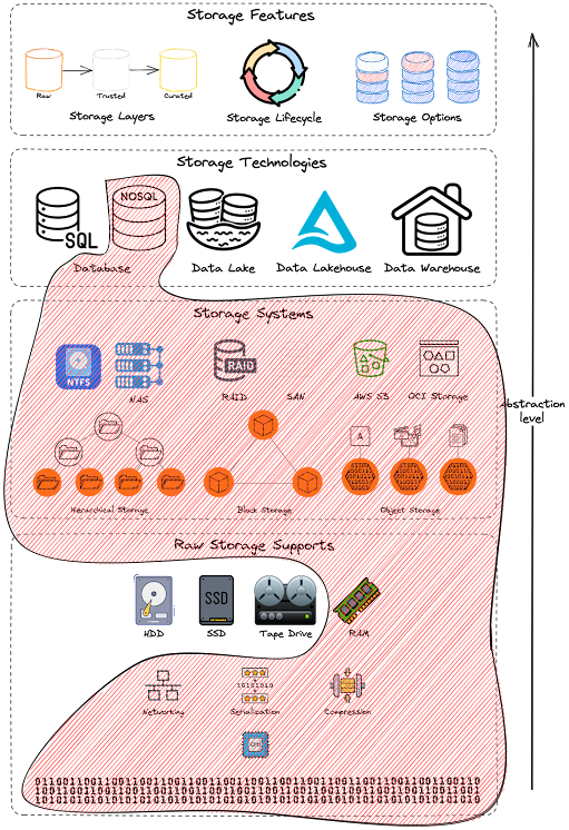 Storage abstractions - Redis Scoped.
To achieve top performance, Redis works in memory. Data is stored and manipulated directly in RAM without disk persistence. Memory is fast and allows Redis to have a very predictable performance. Datasets composed of 10k or 40 million keys will perform similarly. This raw storage support provides faster access to data (at least 1000 times faster than disk access). Pure memory access provides high read and write throughput and low latency. The trade-off is that the dataset cannot be larger than memory.
 Redis: in-memory performance ©ByteByteGo.
Another reason behind the high performance of Redis is a bit unintuitive. A Redis Instance is primarily single-threaded. Multi-threaded applications require locks or other synchronization mechanisms. They are notoriously hard to reason about. In many applications, the added complexity is bug-prone and sacrifices stability, making it difficult to justify the performance gain. In the case of Redis, the single-threaded code path is easy to understand.
However, it might become problematic when it comes to handling many thousands of incoming requests and outgoing responses simultaneously with a single-threaded codebase. Processing time in Redis is mainly wasted on waiting for network I/O; thus, bottlenecks might arise.
This is where I/O multiplexing comes into the picture. With I/O multiplexing, the operating system allows a single thread to wait on many socket connections simultaneously and only returns sockets that are readable.

A drawback of this single-threaded design is that it does not leverage all the CPU cores available in a node. However, it is not uncommon for modern workloads to have several Redis instances running on a single server to utilize more CPU cores. This is why Redis Enterprise provides a symmetric shared-nothing architecture to completely separate the data path and control & management path, leveraging multiple Redis instances to be hosted in the same node. It also allows a multi-threaded stateless proxy to hide the cluster’s complexity, enhancing the security (SSL, authentication, DDoS protection) and improving performance (TCP-less, connection management, and pipelining).
Finally, the third reason why Redis is fast is the native data structures provided by Redis. Code-wise, in-memory data structures are much easier to implement than their on-disk counterparts. This keeps the code simple and contributes to Redis’ rock-solid stability. Furthermore, since Redis is an in-memory database, it could leverage several efficient low-level data structures without worrying about persisting them to disk efficiently - linked list, skip list, and hash table are some examples. I will dive deep into each data structure and what level of complexity it offers.

Redis Most Common Use-Cases
In this section, we will discover the versatility of Redis by discussing the top use cases that have been battle-tested in production at various companies and at various scales.
1 - Caching
Redis is an in-memory data structure store, and its most common usage is caching objects to speed up applications. It exploits the memory available on application servers to store frequently requested data. Thus, allows returning frequently accessed data quickly. This reduces the database load and improves the application’s response time. For this purpose, it supports data structures like strings, hashes, lists, sets, and sorted sets. Several patterns exist for caching:
- Cache-Aside (Lazy-Loading): The most common one is Cache-aside or lazy-loading. With this strategy, the application first looks into the cache to retrieve the data. If data is not found (cache miss), the application then retrieves the data from the operational data store directly. Data is loaded to the cache only when necessary (hence lazy-loading). Read-heavy applications can significantly benefit from implementing a cache-aside approach.
- Write-Behind: In this strategy, data is first written to the cache and then is asynchronously updated in the operational data store. This approach improves write performance and eases application development since the developer writes to only one place (Redis).
- Write-Through cache strategy is similar to the write-behind approach, as the cache sits between the application and the operational data store, except the updates are done synchronously. The write-through pattern favors data consistency between the cache and the data store, as writing is done on the server’s main thread. RedisGears and Redis Data Integration (RDI) provide both write-through and write-behind capabilities.
- Read-Through (Read-Replica): In an environment where you have a large amount of historical data (e.g., a mainframe) or have a requirement that each write must be recorded on an operational data store, Redis Data Integration (RDI) connectors can capture individual data changes and propagate exact copies without disrupting ongoing operations with near real-time consistency. CDC, coupled with Redis Enterprise’s ability to use multiple data models, can give you valuable insight into previously locked-up data.

2 - Session Store
Another common use case is to use Redis as a session store to share session data among stateless servers. When a user logs in to a web application, the session data is stored in Redis, along with a unique session ID that is returned to the client as a cookie. When the user makes a request to the application, the session ID is included in the request, and the stateless web server retrieves the session data from Redis using the ID. The session stores are behind the shopping cart you can find on the e-commerce website.

3 - Distributed Lock
Distributed locks are used when multiple nodes in an application need to coordinate access to some shared resource. Redis is used as a distributed lock with its atomic commands like SETNX (SET if Not eXists). It allows a caller to set a key only if it does not already exist. Here’s how it works at a high level:
Client 1 tries to acquire the lock by setting a key with a unique value and a timeout using the SETNX command: SETNX lock "1234abcd" EX 3
- If the key was not already set, the
SETNXcommand returns 1, indicating that the lock has been acquired by Client 1.- Client 1 finishes its work;
- and releases the lock by deleting the key.
- If the key was already set, the
SETNXcommand returns 0, indicating that another client already holds the lock.- In this case, Client 1 waits and retries the
SETNXoperation until the other client releases the lock.
- In this case, Client 1 waits and retries the
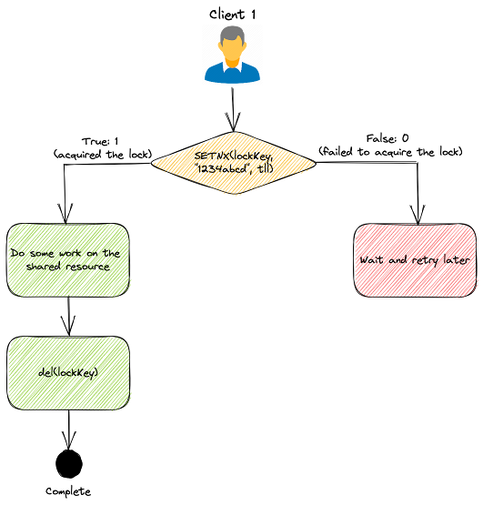 Example of a Distributed Lock implementation.
This simple implementation might be good enough for many use cases, but it is not completely fault-tolerant. For production use, many Redis client libraries provide high-quality distributed lock implementation built out of the box.
4 - Rate Limiter / Counter
Redis strings provide capabilities to manipulate integers with commands like INCR and INCRBY. These commands help you implement counters, for example. The most common usage for Redis-based counters is rate limiters. You can implement one using the strings increment commands on some counters and setting expiration times on those counters. A very basic rate-limiting algorithm works this way:
- The request IP or user ID is used as a key for each incoming request.
- The number of requests for the key is incremented using the
INCRcommand in Redis. - The current count is compared to the allowed rate limit.
- The request is processed if the count is within the rate limit.
- The request is rejected if the count exceeds the rate limit.
- The keys are set to expire after a specific time window, e.g., a minute, to reset the counts for the next time window.

More sophisticated rate limiters like the leaky bucket algorithm can also be implemented using Redis. You can also implement such counters using the HyperLogLog data structure.
5 - Ranking / Gaming Leaderboard
Redis is a delightful way to implement various gaming leaderboards for most games that are not super large-scale. Sorted Sets are the fundamental data structure that enables this. A Sorted Set is a collection of unique elements, each with a score associated with it. The elements are sorted by score. This allows for quick retrieval of the elements by the score in logarithmic time.
 Redis SortedSets ©ByteByteGo.
6 - Message Queue
When you need to store and process an indeterminate series of events/messages, you can consider Redis. In fact, Redis Lists (linked lists of string values) are frequently used to implement Lists, Stacks, LIFO queues, and FIFO queues. In addition, Redis also uses the lists to implement Pub/Sub messaging architectures.
 Push and Pop into/from Redis Lists.
In the publishers/subscribers (Pub/Sub) paradigm, senders (publishers) are not programmed to send their messages to specific receivers (subscribers). Instead, published messages are characterized into channels without knowledge of what (if any) subscribers there may be. Likewise, subscribers express interest in one or more channels and only receive messages that are of interest without knowing what (if any) publishers exist. This decoupling of publishers and subscribers enables the communication between different components or systems in a loosely-coupled manner, allowing greater scalability and more dynamic network topology.
 Publisher/Subscriber Paradigm.
Redis also provides a specific data structure, called Redis Streams, that acts like an append-only log. You can use streams to record and simultaneously syndicate events in real-time. Examples of Redis stream use cases include:
- Event sourcing (e.g., tracking user actions, clicks, etc.)
- Sensor monitoring (e.g., readings from devices in the field)
- Notifications (e.g., storing a record of each user’s notifications in a separate stream)

7 - Social Networking
We live in a connected world, and understanding most relationships requires processing rich sets of connections to understand what’s really happening. Social media networks are graphs in which relationships are stored natively alongside the data elements (the nodes) in a much more flexible format. This is where RedisGraph comes in.

RedisGraph is a graph database built on Redis. This graph database uses GraphBlas under the hood for its sparse adjacency matrix graph representation. It adopts the Property Graph Model and has the following characteristics:
- Nodes (vertices) and Relationships (edges) may have attributes;
- Nodes can have multiple labels;
- Relationships have a relationship type;
- Graphs represented as sparse adjacency matrices;
- OpenCypher with proprietary extensions as a query language;
- Queries are translated into linear algebra expressions.
Everything about the system is optimized for traversing through data quickly, with millions of connections per second. RedisGraph can also be used for recommendation engines to Rapidly find connections between your customers and their preferences.
8 - Full-Text Search
Full-text search refers to searching some text content inside extensive text documents and returning results that contain some or all of the words from the query. While traditional databases are great for storing and retrieving general data (exact matching), performing full-text searches has been challenging. This is why Redis created the RedisJSON module to store JSON documents natively. This module allowed Redis to store, update, and retrieve all or a few JSON values in a Redis database, similar to any other Redis data type.
 Google Search Engine - Autocompletion.
RedisJSON works seamlessly with the RediSearch module to create secondary indexes and query JSON documents. In addition, RediSearch enables multi-field queries, aggregation, exact phrase matching, numeric filtering, geo-filtering, and similarity semantic search on top of text queries.
9 - Similarity Search
Another advantage of using RediSearch is the similarity search feature it provides. Similarity search allows finding data points that are similar to a given query feature in a database. The most popular use cases are Vector Similarity Search (VSS) for recommendation systems, image and video search, natural language processing, and anomaly detection. For example, if you build a recommendation system, you can use VSS to find (and suggest) products that are similar to a product in which a user previously showed interest or looks similar to another product you already bought.

It is also used to train Large Languages Models that use machine learning algorithms to process and understand natural languages. For example, OpenAI leveraged Redis as a vector database to store embeddings and performs vector similarity calculations to find similar topics, objects, and content for chatGPT.
Redis Data Structures
In this section, I’ll quickly review the native data structures that help you address the use cases presented above.
1 - Strings
Redis strings store sequences of bytes, including text, serialized objects, and binary arrays. As such, strings are the most basic Redis data type. They’re often used for caching but also support additional functionality that lets you implement atomic counters or locks and perform bitwise operations. Strings combined with TTL and eviction policy are the preferred structure when implementing a cache.
 A Redis String.
Most string operations have algorithmic complexity of O(1), which means they’re highly efficient. However, be careful with the SUBSTR, GETRANGE, and SETRANGE commands, which can be O(n). These random-access string commands may cause performance issues when dealing with large strings. A single Redis string can be a maximum of 512 MB by default. If you’re storing structured data, you may also want to consider Hashes.
2 - Hashes
Redis hashes are record-structured types as collections of field-value pairs. You can use hashes to represent basic objects and store groupings of counters, among other things. Most Redis hash commands have algorithmic complexity of O(1). A few commands - such as HKEYS, HVALS, and HGETALL - are O(n), where n is the number of field-value pairs. Every hash can store up to 4,294,967,295 (232 - 1) field-value pairs. Note that each field name and value is a Redis string limited to 512 MB. Therefore, the maximum size of a hash can reach up to 4,294PB (aka. (232 -1) x 2 x 512MB). In practice, your hashes are limited only by the overall memory on the VMs hosting your Redis deployment.

3 - Set
A Redis set is an unordered collection of unique strings (members). You can use Redis sets to efficiently track unique items (e.g., track all unique IP addresses accessing a given blog post), represent relations (e.g., the set of all users with a given role), or perform cross-sets operations such as intersection, unions, and differences. The max size of a Redis set is 4,294,967,295 (232 - 1) unique members, which means a maximum size of 2,147PB (4,294,967,295 x 512MB) per set.
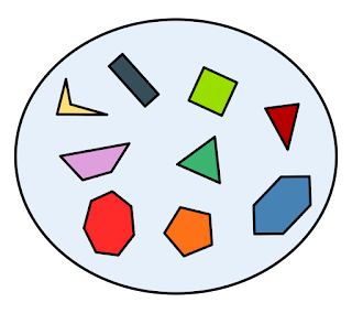 A Set of unique elements.
Most set operations, including adding, removing, and checking whether an item is a set member, are O(1). This means that they’re highly efficient. However, for large sets with hundreds of thousands of members or more, you should exercise caution when running the SMEMBERS command. This command is O(n) and returns the entire set in a single response. As an alternative, consider the SSCAN, which lets you retrieve all set members iteratively.
Sets membership checks on large datasets (or streaming data) can use a lot of memory. If you’re concerned about memory usage and don’t need perfect precision, consider a Bloom filter as an alternative to a set. Moreover, if you use Redis sets as an indexing mechanism and need to perform queries on your set’s members, consider RediSearch and RedisJSON.
4 - SortedSet
Redis sorted set is a collection of unique strings (members) ordered by an associated score. When more than one string has the same score, the strings are ordered lexicographically. The max size of a Redis sorted set is 4,294,967,295 (232 - 1) unique members, which means a maximum size of 2,147PB (4,294,967,295 x 512MB) per sorted set.
Most sorted set operations are O(log(n)), where n is the number of members. You must consider running the ZRANGE command might return large values (e.g., in the tens of thousands or more). This command’s time complexity is O(log(n) + m), where m is the number of results returned.
Redis sorted sets can easily maintain ordered lists of the highest scores in a massive online game (leaderboards), you can use a sorted set to build a sliding window rate limiter to prevent excessive API requests, and you can use them to store time series, using a timestamp as a score.
 A Redis Sorted Set (ZSet).
They are also often used as secondary indices for range queries. For example, to get all the customers with a specific name (e.g., “Amine”) with ages between 30 and 50. Redis sorted sets are sometimes used for indexing other Redis data structures. If you need to index and query your data, consider RediSearch and RedisJSON.
5 - Lists
Redis lists are linked lists of string values. A list can store up to 4,294,967,295 (232 - 1) elements and keep the items ranked. Which means a maximum size of 2,147PB (4,294,967,295 x 512MB) per list. Redis lists are frequently used to implement stacks and queues. Redis can add or remove an item at the bottom (LPUSH, LPOP) or at the top of a list (RPUSH, RPOP).
They also support blocking commands such as “get next item if there is one, or wait until there is one” (BLPOP, BLMOVE). Redis can also execute cross-list commands to get and remove an item from a list and add it to another list (BRPOPLPUSH). List operations that access its head or tail are O(1), which means they’re highly efficient. However, commands that manipulate elements within a list are usually O(n). Examples of these include LINDEX, LINSERT, and LSET. So exercise caution when running these commands, mainly when operating on large lists.
Consider Redis streams as an alternative to lists when you need to store and process an indeterminate series of events.
6 - Streams
Redis stream is a data structure that acts like an append-only log. You can add new entries, they will be timestamped and stored, but you can not delete or alter an existing entry. Redis Streams is often used to record and simultaneously syndicate events in real time. Therefore, Redis Streams can be convenient for implementing data synchronization on a weak link, data ingestion from IoT devices, event logging, or a multi-user chat channel.
Then, you can execute a range query such as “get all records between yesterday and today.” Redis generates a unique ID for each stream entry. You can use these IDs to retrieve their associated entries later or to read and process all subsequent entries in the stream.
Streams were made to store unbounded events, so theoretically, your streams are limited only by the overall memory on the VMs hosting your Redis deployment. However, each event up to 4,294,967,295 (232 - 1) field-value pairs. Note that each field name and value is a Redis string limited to 512 MB.
Adding an entry to a stream is O(1). Accessing any single entry is O(n), where n is the length of the ID. Since stream IDs are typically short and of a fixed length, this effectively reduces to a constant time lookup. This was made possible only because streams were implemented using radix trees.
You can subscribe to a stream to receive each new record in real-time, subscribe to a past stream to resume a lost connection and ask the stream to distribute the records to a consumer group to distribute the load, with acknowledgments. If all entries are the same, Redis Streams stores field names once, so there is no need to store them for new entries.
Redis streams support several trimming strategies (to prevent streams from growing unbounded) and more than one consumption strategy (see XREAD, XREADGROUP, and XRANGE).
7 - Geospatial Indexes
Redis geospatial indexes let you store coordinates and search for them. This data structure is useful for finding nearby points within a given radius or bounding box and calculating distances.

This data structure is not really a new native data structure but a derived data structure. Internally, this structure uses a sorted set to store the items and uses a geo-hash calculated from the coordinates as a score. The difference between two geo-hashes is proportional to the physical distance between the coordinates used to compute these geo-hashes. It also has the same properties as the sorted set, with additional commands to calculate distances between points or retrieve items by distance.
8 - Bitmap
Another derivative data structure in Redis is the Bitmap. Redis bitmaps are an extension of the string data type that lets you treat a string like a bit vector. You can also perform bitwise operations on one or more strings, such as AND, OR, and XOR. For example, suppose you have 100 movement sensors deployed in a field labeled 0-99. You want to quickly determine whether a given sensor has detected a movement within the hour. All you can do is create a bitmap with a key for each hour and let the sensors set it with their ID when they capture a movement. Then, you can simply see which sensor was pinging in your field by displaying the bitmap.
 A Bitmap presenting the activated sensors in the field.
9 - Bitfield
Redis bitfields let you set, increment, and get integer values of arbitrary bit length. For example, you can operate on anything from unsigned 1-bit integers to signed 63-bit integers. These values are stored using binary-encoded Redis strings. This is a huge storage saver: you can hold values in the 0-8 range, but you will need only 3 bits per value.
Bitfields support atomic read, write, and increment operations, making them a good choice for managing counters and similar numerical values (e.g., configuration, settings…).
10 - HyperLogLog
HyperLogLog is a data structure that estimates the cardinality of a set. Usually, when you need to count thousands or millions of unique elements, you typically need also to store the counted elements to count them only once. On the other hand, HyperLogLog will only keep the counter in a 12KB record, and It will never use more than 12 KB.
As a probabilistic data structure, HyperLogLog trades perfect accuracy for efficient space utilization. The HyperLogLog implementation uses up to 12 KB and provides a standard error of 0.81%.
The HyperLogLog can estimate the cardinality of sets with up to 18,446,744,073,709,551,616 (246) members. Writing (PFADD) to and reading from (PFCOUNT) the HyperLogLog is done in constant time and space. Merging HLLs is O(n), where n is the number of sketches.
If you want to count unique visitors on your website, you will probably use the visitors’ IP addresses as a counting criterion. For example, Hyperloglog can tell you that you have one million unique IP addresses with a 0.81% accuracy. Still, it will only use 12KB of memory instead of 4MB to store one million IP addresses.
11 - Redis Bloom
There exist other probabilistic data structures in Redis. They are grouped in a module called RedisBloom which contains a set of useful probabilistic data structures. Probabilistic data structures allow developers to control the accuracy of returned results while gaining performance and reducing memory. These data structures are ideal for analyzing streaming data and large datasets. Besides the HyperLogLog, you can use:
- Bloom filter and Cuckoo filter: These filters check whether an element already appears in a large dataset. Bloom filter typically exhibits better performance and scalability when inserting items (so if you’re often adding items to your dataset, then a Bloom filter may be ideal). Cuckoo filters are quicker on check operations and also allow deletions.
- Top-K: indicates the top k most frequent values in a dataset.
- t-digest can indicate which fraction (percentage) of the dataset values are smaller than a given value. For example, you can use t-digest to efficiently estimate percentiles (e.g., the 50th, 90th, and 99th percentile) when your input is a sequence of measurements (such as temperature or server latency). And that’s just one example; we explain more of them below.
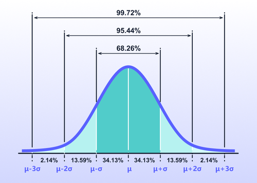 Redis Bloom (t-digest) calculating confidence levels.
These data structures may help in several scenarios: predictive maintenance, network traffic monitoring, or online gaming analysis are a few examples where you can use RedisBloom data structures.
12 - Extended Data Structures with Redis Modules
Redis modules make it possible to extend Redis functionality using external extensions, rapidly implementing new Redis commands and data structures with features similar to what can be done inside the core itself. Modules can leverage all the underlying Redis core features, such as in-memory storage, existing data structure usage, persistency, high availability, data distribution with sharding, etc. The most common modules extending the core data structures of Redis are RedisJSON, RedisGraph, and Redis TimeSeries:
-
The RedisJSON module provides JSON support for Redis. RedisJSON lets you store, update, and retrieve JSON values in a Redis database, similar to any other Redis data type. RedisJSON also works seamlessly with RediSearch to let you index and query JSON documents.
RedisJSON stores JSON values as binary data after deserializing them. This representation is often more expensive, size-wise, than the serialized form. The RedisJSON data type uses at least 24 bytes (on 64-bit architectures) for every value. As Redis Strings, a JSON object can be a maximum of 512 MB.
A JSON value passed to a command can have a depth of up to 128. If you pass a JSON value to a command containing an object or an array with a nesting level of more than 128, the command returns an error. Creating a new JSON document (JSON.SET) is an O(M+N) operation where M is the size of the original document (if it exists) and N is the size of the new one.
-
RedisGraph is a graph database developed from scratch on top of Redis, using the new Redis Modules API to extend Redis with new commands and capabilities. Depending on the underlying hardware results may vary. However, inserting a new relationship is done in O(1). RedisGraph can create over 1 million nodes in under half a second and form 500K relations within 0.3 of a second.
-
Redis TimeSeries is a Redis module that adds a time series data structure to Redis. It allows high volume inserts, low latency reads, query by start time and end-time, aggregated queries (min, max, average, sum, range, count, first, last, standard deviations, variances) for any time bucket, configurable maximum retention period, and time-series downsampling/compaction.
A time series is a linked list of memory chunks. Each chunk has a predefined size of 128 bits (64 bits for the timestamp and 64 bits for the value), and there is an overhead of 40 bits when you create your first data point. Most string operations have algorithmic complexity of O(1), which means they’re highly efficient.
Summary
In this article, We discovered that fundamental design decisions made by the developers more than a decade ago were behind Redis’s performance, thus answering the question: Why is Redis so fast?
We discovered some of Redis’ top use cases that have been battle-tested in production at various companies and at various scales. Then, I introduced the native data structures of Redis and the extended ones implemented with the Redis Modules. I also presented the algorithmic complexity (Big O notation) of read/write operations of each data structure, the well-known limitations, and the maximum storage limit of each. This is an illustrated recap of this article:

Redis is very versatile: there are many different ways to use it. The only limit is your creativity.
References
- Redis Data Types, Redis.io
- Redis 03 - Native datastructures (1/2), François Cerbelle’s Blog
- Redis 03 - Native datastructures (2/2), François Cerbelle’s Blog
- “Why is redis so fast?”, ByteByteGo Blog
- “Announcing ScaNN: Efficient Vector Similarity Search”, Google Research Blog