
Up to this stage, data has primarily been passed from one place to another or stored. In this article, you’ll learn how to make it useful. Data Processing involves transforming raw data into valuable insights through analysis techniques like machine learning algorithms or statistical models depending on what type of problem needs solving within an organization’s context.
Data processing is the core of any data architecture, and we’ve seen in the last posts that choosing the right data architecture should be a top priority for many organizations. The aim here is not only accuracy but also efficiency since this stage requires significant computing power, which could become costly over time without proper optimization strategies employed.
In this post, we will cover data processing with the different stages that compose it. We will see that while data is going further in these stages, it gains in value and can offer better insights for decision-making.
1 - Data Preparation
Once the data is collected, it then enters the data preparation stage. Data preparation, often referred to as “pre-processing,” is the stage at which raw data is cleaned up and organized for the following stages of data processing. During preparation, raw data is diligently checked for any errors. This step aims to discover and eliminate bad data (redundant, incomplete, or incorrect data) and create high-quality data for the best data-driven decision-making.
76% of data scientists say that data preparation is the worst part of their job, yet a mandatory task to perform carefully. This is because efficient, accurate business decisions can only be made with clean data.
Data preparation helps catch errors and raise alerts about data quality before processing. After data has been moved from its original source, these errors become more challenging to understand and correct. Data preparation allows also to produce of top-quality data. As a result, top-quality data can be processed and analyzed more quickly and efficiently, leading to accurate business decisions.
Data Discovery
The data preparation process begins with finding the right data. Either added ad-hoc or came from an existing data catalog, data should be gathered and its attributes discovered and shared in a data catalog. The first step of data preparation is thus data discovery (or data cataloging).
According to Gartner, Augmented Data Catalogs 2019: “A data catalog creates and maintains an inventory of data assets through the discovery, description, and organization of distributed datasets. The data catalog provides context to enable data stewards, data/business analysts, data engineers, data scientists, and other lines of business (LOB) data consumers to find and understand relevant datasets to extract business value. Modern machine-learning-augmented data catalogs automate various tedious tasks involved in data cataloging, including metadata discovery, ingestion, translation, enrichment, and the creation of semantic relationships between metadata.’’
Data is a valuable asset, but its full potential can only be unlocked when users are able to comprehend and transform it into meaningful information. In the era of big data, organizations cannot afford to leave their business users dependent on IT professionals or data analysts to help understand large volumes of generated data. Instead, it serves as a single source of reliable information that gives viewers insight into all available organizational assets, making it essential for businesses who wish to become more informed with their decisions by leveraging relevant insights from collected datasets faster than ever before possible.
Data catalogs focus on organizing different types of assets within one platform while connecting related metadata together so that consumers can easily search through defined categories, ultimately leading them toward smarter decision-making processes without prior knowledge about the underlying dataset itself.
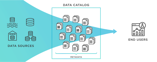 Data catalog.
Data Cleaning
In computer science, the phrase “Garbage In, Garbage Out” states that the quality of an output depends on its inputs. Despite this simple yet self-evident concept being widely accepted, many modern data teams still experience difficulties with their source data’s quality leading to pipeline failures. In addition, data quality issues cause frustration among data consumers. Large enterprises are neither immune from these issues due to a lack of properly addressing data quality.
Data cleaning (aka data cleansing or scrubbing) is a critical component of the preparation process, as it eliminates faulty information and fills in gaps. This includes eliminating unnecessary details, removing duplicates and corrupted/incorrectly formatted data, correcting outliers, filling empty fields with appropriate values, and masking confidential entries. After this step has been completed successfully, validation must occur to ensure that no errors have occurred during the cleansing procedure. If an issue arises at this stage, it must be addressed before moving forward.
To establish a successful data cleaning process, your organization should begin by outlining the techniques used for each data type. For instance, you can follow these steps (non-exhaustive) to map out a framework for your organization.
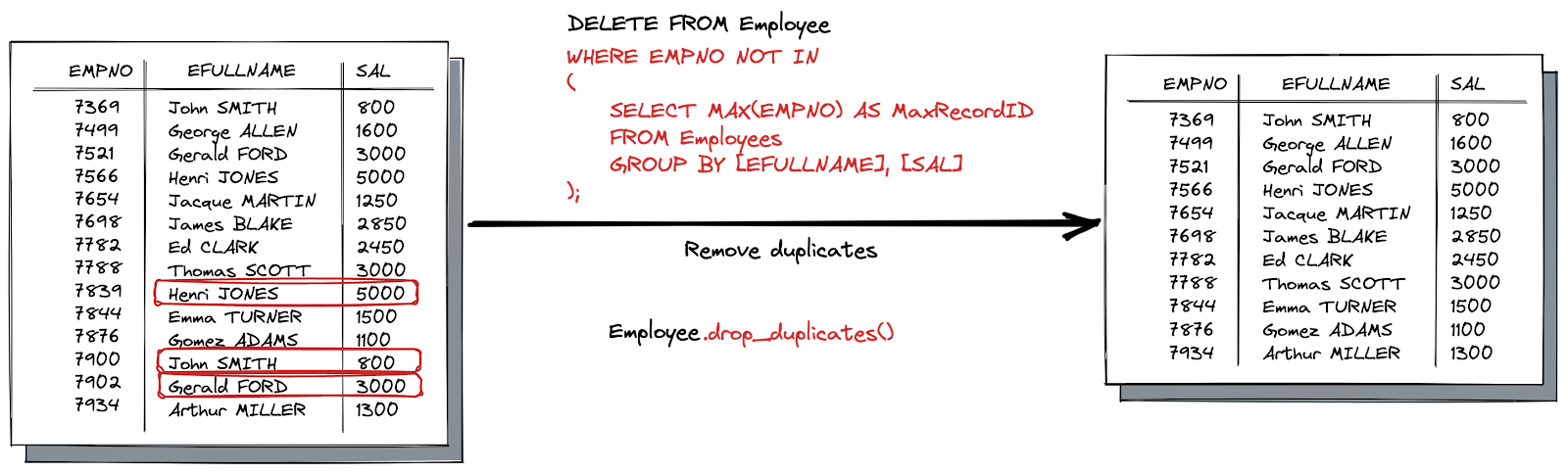
- Remove duplicate or irrelevant observations: To remove unwanted observations from a dataset, one should first identify and eliminate any duplicate or irrelevant observations. This can be done by examining the data for similarities between records that may indicate duplication and filtering out observations that do not fit into the specific problem being analyzed. Doing so will help to create an efficient dataset with only relevant information that is more manageable and performant when it comes time to analyze the data.
- Fix structural errors: Structural errors occur when data is measured or transferred and strange naming conventions, typos, or incorrect capitalization are noticed. These inconsistencies can lead to mislabeled categories or classes; for instance, both “N/A” and “Not Applicable” may appear but should be treated as the same category.
- Filter unwanted outliers: Occasionally, a single observation may stand out from the rest of the data and not seem to fit in with what is being analyzed. If there is an acceptable reason for eliminating it, such as incorrect information entry, this can improve the accuracy of your results. However, outliers could also be significant; they might confirm or disprove the theories you are exploring. Therefore, before discarding any unusual values that appear in your dataset, make sure to investigate their validity first. If they turn out to be irrelevant or erroneous, then consider removing them from consideration.
- Handle missing data: Missing data cannot be overlooked, as many algorithms will not accept it. To address this issue, there are a few potential solutions; however, none of them is perfect. One option is to remove observations that contain missing values, but doing so can lead to the loss of information. Another approach would involve filling in the gaps with assumptions based on other entries, which could compromise accuracy and integrity. Lastly, one might consider altering how the data is used in order to effectively work around null values without sacrificing its quality or reliability.
- Data contracts can also offer a practical answer to clean and align data according to specific agreements long before it is consumed.
In the table below, you can find the most frequent data issues, with some examples and how to deal with them.
| Data Quality Issue | Description | Examples | Solutions |
|---|---|---|---|
| Missing Data | Reason of Missing Values: 1.Information not collected from the source, 2.Attribute not applicable to all cases. |
Empty Fields. | The solutions applied will depend on the amount of missing data, the attributes with the missing data, and the category of missing data: - Drop the observations with missing data (remove the Rows); - Fill in the missing data (Mode for Categorical data, Means or Median for Numerical Values); - Ignore the attribute with missing data (remove the Columns). |
| Outliers | Data objects having characteristics that are considerably different than most of the other data objects in the dataset. | Having Millions while most of the data values are less than 10. | The solutions applied will depend on the Outlier nature: - A measurement error or data entry error. Correct the error if possible. If you can’t fix it, remove that observation because you know it’s incorrect; - Not a part of the population you are studying (i.e., unusual properties or conditions), you can legitimately remove the outlier; - A natural part of the population you are studying, you should not remove it. Analyses the origin of the value and considers the trade-offs to keep the outlier. |
| Noise | Refers to modification of original values with the additional meaningless information. | Multiple Rows are filled by default values. | Drop Noise |
| Contaminated Data | All the data exist but in the wrong field or are inaccurate. | Phone number in the Name Field. | Data Contracts (schema enforcement) |
| Inconsistent Data | Discrepancies in the same information across the dataset. | - Same person with multiple name spelling; - Discrepancies in the unit of measure (Euros and Dollars in the same field). |
Data Contracts (semantics enforcement) |
| Invalid Data | Data exists but is meaningless in the context. | Inventory available units displaying a negative value. | Data Contracts (semantics enforcement) |
| Duplicate Data | Reason for Duplicates: Merge of Data from Heterogenous Sources. | The same person present in multiple rows. | Drop Duplicates |
| Datatype Issues | Data exists but with the wrong Data archetype. | Having Dates or Numbers in String Fields. | Data Contacts (schema enforcement) |
| Structural Issues | The data structure is not as expected. | - Expecting 10 fields and getting only 3; - Expecting a specific Structure Order and getting a different order. |
Data Contacts (schema enforcement) |
At the end of the data cleaning process, you should be able to answer these questions as a part of basic validation:
- Does the data make sense?
- Does the data follow the appropriate rules for its field?
- Does it prove or disprove your working theory, or bring any insight to light?
- Can you find trends in the data to help you form your next theory?
- If not, is that because of a data quality issue?
False conclusions because of incorrect or “dirty” data can inform poor business strategy and decision-making. Erroneous conclusions can lead to an embarrassing moment in a reporting meeting when you realize your data doesn’t stand up to scrutiny. Before you get there, creating a culture of quality data in your organization is important. To do this, you should document the tools you might use to make this culture and what data quality means to you.
Once prepared, the data can be stored or leveraged to a trusted storage zone (in multi-tier storage), clearing the way for processing and analysis to take place.
Data Contract & SLA
Data Contracts are SLA-driven agreements between everyone in the data chain of value. It can involve the data producers who own the data and the data engineers that implement the data pipelines. It can involve the data engineers and the data scientist that require a specific format with a specific number of features, or simply between the data consumers who understand how the business works and the upstream actors involved in the data journey. The aim of these contracts is to generate well-modeled, high-quality, trusted, and real-time data.
Instead of data teams passively accepting dumps of data from production systems that were never designed for analytics or Machine Learning, Data Consumers can design contracts that reflect the semantic nature of the world composed of Entities, events, attributes, and the relationships between each data object. For instance, this abstraction allows data engineers to stop worrying about production-breaking incidents when a data source changes its schema.
Data Contracts are a cultural shift towards data-centric collaboration, and their implementation must meet specific basic requirements to be effective. These include enforcing contracts at the producer level, making them public with versioning for change management, covering both schemas and semantics (including descriptions, value constraints, etc.), and allowing access to raw production data in limited sandbox capacity. This reduces tech debt and tribal knowledge within an organization, leading to faster iterations overall.
Data Contracts should hold the schema of the data being produced and its different versions. Thus consumers should be able to detect and react to schema changes and process data with the old schema. The contract should also hold the semantics: for example, what entity a given data point represents. Similarly to the schema, the semantics can evolve over time and might represent an issue if it is broken (data inconsistency).
In addition, data contracts must contain the level of agreements (SLA) metadata: is it meant for production use? How late can the data arrive? How many missing values could be expected for specific fields in a given period?…

Schemas, Semantics, SLA, and other metadata (e.g., those used for data lineage) are registered by data sources into a central data contract registry. Once data is received by an event processing engine, it validates it against parameters set in the data contract.
Data that do not meet the contract requirements are pushed to a Dead Letter Queue for alerting and recovery: Consumers and Producers are both alerted for any SLA noncompliance, and invalidated data can be re-processed with a recovery logic (logic on how to fix invalidated Data). Data that meet the contract are pushed to the serving layer.
2 - Data Formatting
The clean data is then entered into its destination (perhaps a CRM like Salesforce or a data warehouse like Redshift) and should be formatted into a format that it can understand and is efficient to process. Data formatting is the first stage in which cleaned data takes the form of usable information.
In data processing, there are various file formats to store datasets. Each format has its own advantages and disadvantages depending on the use cases it is intended for. Therefore, it is important to understand their specificities when selecting a particular format type. For instance, CSV files are easy to comprehend but lack formalism; JSON is preferred in web communication while XML may also be used; AVRO and Protocol Buffers work well with streaming processing; ORC and Parquet offer improved performance in analytics tasks due to column storage capabilities. Furthermore, Protocol Buffers form the basis of gRPC, which powers Kubernetes ecosystem applications.
Formatting Considerations
Many considerations have to be taken into account for choosing a data format and the underlying technology for its storage (aka file format). In this section, I will describe the most popular and representative data formats regarding their main characteristics, for example, storage mode, query types, processing usages, etc. The goal here is to provide a way to compare the most popular data formats depending on what you want to perform at this stage. The main characteristics we retained for comparison are:
- Encoding: While both binary and text files contain data stored as a series of bits (binary values of 1s and 0s), the bits in text files represent characters (ASCII code), while the bits in binary files represent custom data. Text-based encodings are advantageous because they can be read and modified by the end user with a text editor. Furthermore, these files tend to have smaller storage footprints due to compression. On the other hand, binary encodings require specialized tools or libraries for creation and consumption; however, their data serialization is optimized for better performance while processing data.
- Data type: Some formats do not permit the declaration of multiple data types. These types are divided into two categories: scalar and complex. Scalar values contain a single value, such as integers, booleans, strings, or nulls, whereas complex values consist of combinations of scalars (e.g., arrays and objects). Declaring type is beneficial because it allows consumers to differentiate between numbers and strings, for example, or distinguish a null from the string “null.” When encoded in a binary form, this distinction results in significant storage optimization: For example, the string “1234” requires four bytes, while boolean 1234 only requires two.
- Schema enforcement: The schema stores each attribute’s definition and its types. Unless your data is immutable, you will need to consider schema evolution in order to determine if your data’s structure changes over time. Schema evolution enables updating the schema used for writing new data while still being compatible with the old schemas that were previously used (backward compatibility).
- Row vs. column storage: In row-based storage, data is organized and stored in rows. This architecture makes it easy to add new records quickly and facilitates simultaneous access or processing of an entire row of data. It is commonly used for Online Transactional Processing (OLTP) systems that process CRUD queries at a record level. OLTP transactions are usually very specific tasks involving one or more records, with the main emphasis being placed on maintaining data integrity in multi-access environments while achieving high numbers of transactions per second. Inversely, column-based storage is most useful when performing analytics queries requiring only a subset of columns examined over large data sets. This approach, known as OLAP (OnLine Analytical Processing), has played an important role in business intelligence analytics and Big Data processing. Storing data in columns instead of rows avoids the excessive time needed to read irrelevant information across a dataset by ignoring all the data that doesn’t apply to a particular query. It also provides a greater compression ratio due to aligning similar types of data and optimizing null values for sparse columns. For example, if you wanted to know the average population density in cities with more than one million people using row-oriented storage, your query would access each record from the table (all its fields). At the same time, columnar databases reduce this amount, significantly improving performance times.
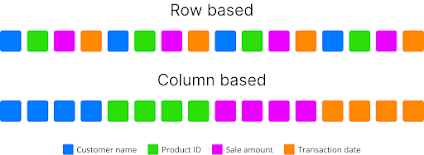 Grouping records by properties.
- Splittable: In a distributed system like Hadoop HDFS, it is essential to have a file that can be broken down into multiple parts. This allows for the data processing in the system to be distributed among these chunks, thus being able to scale the processing to infinite. Being able to start reading from any point within a file fully uses Hadoop’s distributed capabilities. Users must manually divide their files into smaller pieces to enable parallelism if the file format does not permit splitting.
- Data Compression: A system’s performance is largely determined by its slowest components, often the disks. Compression can reduce the size of datasets stored and thus decrease read IO operations and speed up file transfers over networks. Column-based storage offers higher compression ratios and better performance than row-based storage due to similar pieces of data being grouped together; this is especially effective for sparse columns with many null values. When comparing compression ratio, one must also consider the original size of each individual file. E.g., it would be unfair to compare JSON versus XML without considering that XML tends to have a more significant initial footprint than JSON does. Various types of compression algorithms are available depending on factors such as desired level of compression, speed/performance requirements, whether or not they’re splittable, etc.
- Data velocity: Batch processing involves simultaneously reading, analyzing, and transforming multiple records. In contrast, stream processing works in real-time to process incoming records as they arrive. It is possible for the same data set to be processed both through streaming and batch methods. For example, financial transactions received by a system could be streamed instantly for fraud detection while also being stored periodically in batches so that reports can be prepared later. To achieve this goal, one or two file formats might need to exist between the format of the data arriving over the wire and what is eventually stored in Data Warehouse/Data Lake systems.
- Ecosystem and Integration: It is advisable to adhere to the conventions and customs of an ecosystem when selecting between multiple options. For instance, Parquet should be used on Cloudera platforms. In contrast, ORC with Hive should be preferred for Hortonworks ones, as it will likely result in a smoother integration process and more helpful documentation/support from the community.
File formats
We will focus on some of the more common data formats, providing examples to help data engineers retrieve their desired information. We cannot examine all available formats due to the vast number of formats available. Instead, we will tackle several of the more common formats, providing adequate examples to address the most common data retrieval needs:
1- Delimited Flat Files (CSV, TSV)
Comma-separated values (CSV) and Tab-separated values (TSV) are text file formats that use newlines to separate records and an optional header row. As a result, they can be easily edited by hand, making them highly comprehensible from a human perspective. Unfortunately, neither CSV nor TSV does not support schema evolution; even though the header may sometimes serve as the data’s schema, this isn’t always reliable. Furthermore, their more complex forms cannot be split into smaller chunks without losing relevance due to the lack of any specific character on which splitting could be based.
The differences between TSV and CSV formats can be confusing. The obvious distinction is the default field delimiter: TSV uses TAB, CSV uses a comma, and both use a newline as the record delimiter.
The CSV format is not fully standardized, as its field delimiters can be a variety of characters, such as colons or semicolons. This makes it difficult to parse when the fields contain these exact quotes and even embedded line breaks. Furthermore, data in each field may also be enclosed by quotation marks which further complicates parsing due to potential irrelevant structure regarding sentence beginnings and endings or null values. In contrast, TSV typically uses either tabulation or commas for delimiting without an escape character; this simplifies distinguishing between fields and thus facilitates easier parsing than with CSV files. For this reason, TSV is mainly used in Big Data cases where ease of parsing matters most.
These file formats are prevalent for data storage and transfer. They have excellent compression ratios, making them easy to read and supporting batch and streaming processing. However, neither CSV nor TSV does not support null values, as they are treated the same as empty values. There is no guarantee that files will either be splittable or have schema evolution support.
Despite these drawbacks, delimited text formats remain among the most widely supported formats due to their simplicity with many applications such as Hadoop, Spark, and Kafka…
2- JSON (JavaScript object notation)
JSON is a text-based format that can store data in various forms, such as strings, integers, booleans, arrays, object key-value pairs, and nested data structures. It’s lightweight, human-readable, and machine-readable, making it an ideal choice for web applications. JSON has widespread support across many software platforms, and its implementation is relatively straightforward in multiple languages. Furthermore, the serialization/deserialization process of JSON natively supports this type of data storage.
The main disadvantage of this format is that it cannot be split. To overcome this, JSON lines are often used instead; these contain multiple valid JSON objects on separate lines, each separated by a newline character \n. Since the data being serialized in JSON does not include any newlines, we can use them to divide the dataset into smaller chunks.
JSON is a compressible text-based format used for data exchange and supports batch and streaming processing. It stores metadata with the data and allows schema evolution. However, it lacks indexing as many other text formats. JSON is widely used in web applications such as NoSQL databases like MongoDB or Couchbase, GraphQL APIs, etc.
3- XML (Extensible Markup Language)
XML is a markup language created by W3C that allows humans and machines to read encoded documents. It enables users to create complex or simple languages and establish standard file formats for exchanging data between applications. Like JSON, XML can be used for serialization and encapsulation of information; however, its syntax tends to be more verbose than other text-based alternatives when viewed by human readers.
XML is a verbose file format that supports batch and streaming processing, stores metadata along with the data, and allows for schema evolution. It has drawbacks such as not being splittable due to opening/closing tags at the beginning/end of files, redundant syntax leading to higher storage and transportation costs when dealing with large volumes of data, and difficulties in parsing without an appropriate DOM or SAX parser. Despite these downsides, XML still maintains its presence in many companies due to its long history.
4- AVRO
Apache Avro is a data serialization framework developed as part of Apache’s Hadoop project. It uses row-based storage to serialize data, storing the schema in JSON format, making it easy for any program to read and interpret. Furthermore, the data is stored in binary form, making it compact and efficient. A key feature of Avro is its ability to handle schema evolution; metadata about each record can be attached directly to the data itself. Additionally, Avro supports both dynamic typing (no need to define types in advance) as well as static typing (types are defined before use).
Avro is splittable, compressible, and supports schema evolution. It has a compact storage format which makes it fast and efficient for analytics. Avro schemas are defined in JSON, making them easy to read and parse, while the accompanying data allows full data processing. The downside of Avro is that its data cannot be read by humans, nor does it integrate with every language. However, due to being widely used in many applications such as Kafka or Spark and being an RPC (Remote Procedure Call), Avro remains one of the most popular formats for exchanging information between systems today.
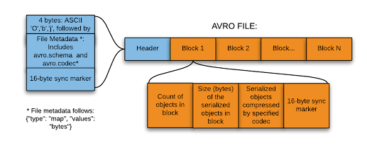 Structure of AVRO format.
5- ProtoBuf (Protocol Buffers)
Protobuf (short for Protocol Buffers) is a binary data serialization format developed by Google in 2008. It is used to efficiently encode structured data in an extensible and language-neutral way, making it ideal for applications such as network communication or storage of configuration settings. Protobuf messages are compact and can be parsed quickly, transferring them over networks faster than other formats like JSON or XML. Unlike Avro, the schema is required to interpret the data. Protocol Buffers format (Protobuf) has advantages such as being fully typed and supporting schema evolution and batch/streaming processing, but it does not support Map Reduce or compression.
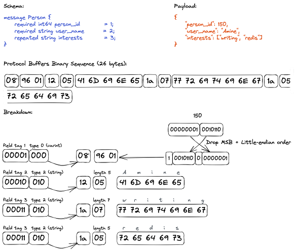 Message encoding using Protocol Buffers.
6- ORC (Optimized Row Columnar)
ORC (short for Optimized Row Columnar) format was developed by Hortonworks in partnership with Facebook. It is a column-oriented data storage system. It consists of stripes containing groups of row data and auxiliary information in a file footer. At the end of the file, a postscript stores compression parameters and the size of the compressed footer. By setting large stripe sizes (e.g., 250 MB as default), HDFS can perform efficient reads on larger files more effectively.
ORC is a highly compressible file format that reduces data size by 75%. It is more efficient for OLAP than OLTP queries and is used mainly for batch processing. However, it does not support schema evolution or adding new data without recreating the file. ORC improves reading, writing, and processing performance in Hive, making it an ideal choice for Business Intelligence workloads.
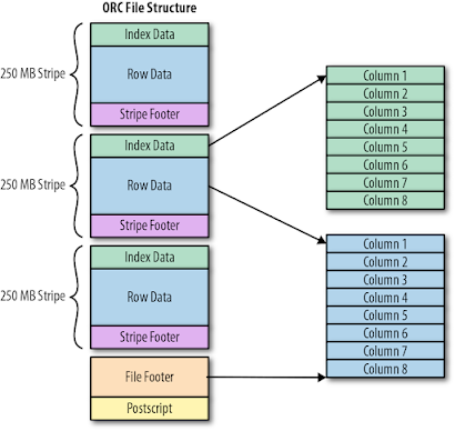 Structure of ORC format.
7- Parquet
Parquet is an open-source file format designed for the Hadoop ecosystem. It was created as a joint effort between Twitter and Cloudera to provide efficient storage of analytics data in a column-oriented fashion, similar to ORC files. Parquet offers advanced compression and encoding schemes that enable it to handle complex data quickly and efficiently when dealing with large volumes of information. In addition, the binary file contains metadata about its content, including the column metadata stored at the end of the file that allows for one-pass writing during creation. Furthermore, Parquet’s optimization makes it ideal for Write Once Read Many (WORM) applications.
Parquet has advantages such as being splittable, allowing better compression and schema evolution due to organizing by columns, and having high efficiency for OLAP workloads. However, it can be challenging to apply updates without deleting and recreating the file again. As a result, parquet is commonly used in ecosystems that require efficient analysis for BI (Business Intelligence) or fast read times with engines like Spark, Impala, Arrow, and Drill.
Databricks recently created a new file format called Delta that uses versioned Parquet files to store data. Apart from the versions, Delta also holds a transaction log to keep track of all the commits made to the table or blob store directory to provide ACID transactions and to leverage the time-machine feature.
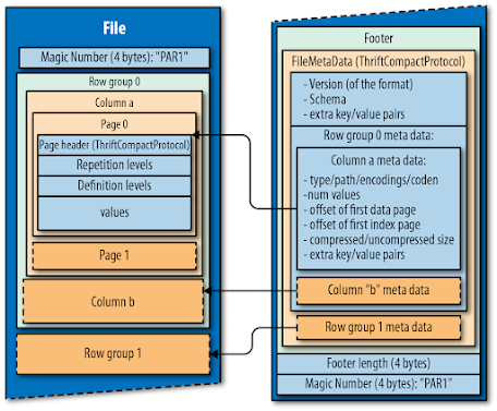 Structure of Parquet format.
The file format selection should be based on the type of query and use cases associated with it. For example, row-oriented databases are typically used for OLTP workloads. At the same time, column-oriented systems are better suited to OLAP queries due to their uniform data types in each column, which allows them to achieve higher compression than row storage formats. JSON line or CSV (if all data types can be controlled) is recommended over XML for text files as its complexity often requires custom parsers. Avro is an ideal choice when flexibility and power are needed for stream processing and data exchange; however, Protocol Buffers may not always be suitable as they cannot split nor compress stored data at rest. Finally, ORC and Parquet formats provide optimal performance for analytics tasks. Choosing the right file format ultimately depends on the specific use case requirements. Hereafter, a summary table for the data formats regarding the selected considerations:
| Attribute\Format | CSV | JSON | XML | AVRO | Protocol Buffers | Parquet | ORC |
|---|---|---|---|---|---|---|---|
| Encoding | Text | Text | Text | metadata in JSON, data in binary | Binary | Binary | Binary |
| Data type | No | Yes | No | Yes | Yes | Yes | Yes |
| Schema enforcement | No | external for validation | external for validation | Yes | Yes | Yes | Yes |
| Schema evolution | No | Yes | Yes | Yes | Yes | Yes | No |
| Storage type | Row-based | Row-based | Row-based | Row-based | Row-based | Column-based | Column-based |
| OLAP/OLTP | OLTP | OLTP | OLTP | OLTP | OLTP | OLAP | OLAP |
| Splittable | Yes (simplest form) | Yes (JSON lines) | No | Yes | No | Yes | Yes |
| Data compression | Yes | Yes | Yes | Yes | No | Yes | Yes |
| Data velocity | Batch & Stream | Batch & Stream | Batch | Batch & Stream | Batch & Stream | Batch | Batch |
| Ecosystems | Very popular | API and web | Enterprise | Big Data and Streaming | RPC and Kubernetes | Big Data and BI | Big Data and BI |
3 - Data Transformation
Organizations generate vast amounts of data on a daily basis, but it is only useful if they can utilize it to gain insights and promote business growth. Data transformation consists of converting and structuring data from one form into a usable form, supporting decision-making processes. Data transformation is utilized when data needs to be changed so that it matches the format and the structure of the target system. This can take place in the so-called data pipelines.
There are several reasons why companies should consider transforming their data: compatibility between disparate sets of information; easier migration from the source format to target format; consolidation of structured and unstructured datasets; enrichment which improves the quality of the collected info; and ultimately achieving consistent, accessible data with accurate analytics-driven predictions.
![]() Transforming data.
Transforming data.
After data preparation (called pre-processing), in which data is identified and understood in its original source format (data discovery), a data transformation pipeline starts with a mapping phase. This involves analyzing how individual fields will be modified, joined, or aggregated to understand the necessary changes that need to be made. Next, the pipeline required to run the transformation process is created using a data transformation platform or tool. Here three approaches can be followed:
- Code-centric tools: analysis and manipulation libraries built on top of general-purpose programming languages (Scala, Java or Python). These libraries manipulate data using the native data structures of the programming language.
- Query-centric tools: use a querying language like SQL (Structured Query Language) to manage and manipulate datasets. These languages can be used to create, update and delete records, as well as query the data for specific information.
- Hybrid tools: implement SQL on top of general-purpose programming languages. This is the case of some libraries like Apache Spark or Apache Kafka that provides a SQL dialect called KSQL.
Organizations often use ETL tools (Extract-Transform-Load), where the transformation can occur following one or many of the above approaches. I’ll create a few data pipelines in the next blog posts using tools in each category.
Data transformation is a critical part of the data journey. This process can perform constructive tasks such as adding or copying records and fields, destructive actions like filtering and deleting specific values, aesthetic adjustments to standardize values, or structural changes that include renaming columns, moving them around, and merging them. Data transformation can be used for :
- Filtering: selects a subset from your dataset (specific columns) that require transformation, viewing, or analysis. This selection can be based on certain criteria, such as specific values in one or more columns, and it typically results in only part of the original data being used. As a result, filtering allows you to quickly identify trends and patterns within your dataset that may not have been visible before. It also lets you focus on particular aspects of interest without sifting through all available information. In addition, this technique can help reduce complexity by eliminating unnecessary details while preserving important insights about the underlying data structure;

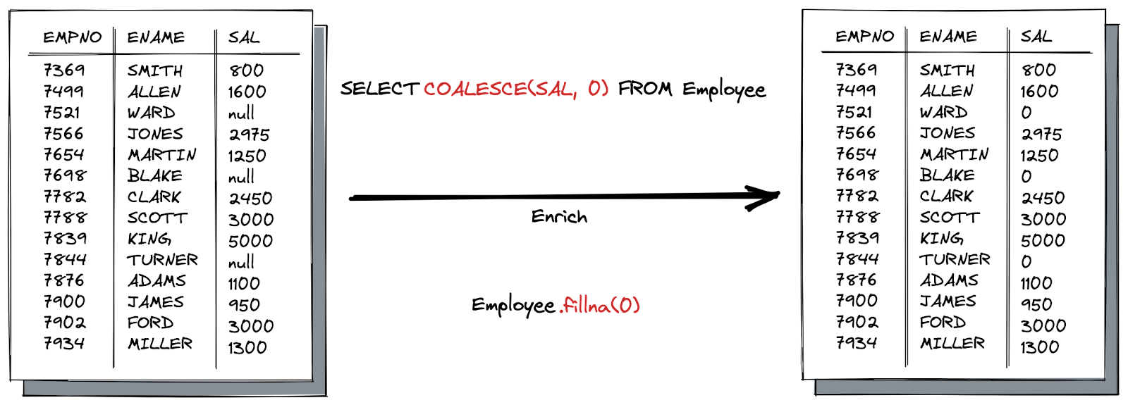
- Enriching: fills out the basic gaps in the data set. This process enhances existing information by supplementing incomplete or missing data with relevant context. It aims to improve accuracy, quality, and value for better results;
- Splitting: where a single column is split into multiple;

- Merging: where multiple columns are merged into one;

- Removing parts of data;
- Joining data from different sources. A data join is when two data sets are combined side-by-side. Therefore at least one column in each data set must be the same. This differs from a union that puts data sets on top of each other, requiring all columns to be the same (or have null values in a column that isn’t common across data sets);

There are nine types of joins: inner, outer, left outer, right outer, anti-outer, anti-left, anti-right, and cross-join:
- An inner join takes the rows of data where both sets have fields in common. Any rows with no shared values between the two datasets on their joined column won’t be included.
- An outer join will keep all data from both data sets. Rows that are common across data sets will have columns filled from both data sets, whereas rows without commonality will fill the blanks in with NULL values.
- The left outer join combines two data sets, taking all the rows shared between them and any remaining rows from the set on the left. Any right-hand columns without corresponding rows in the other dataset will be filled with NULL values.
- The right outer join combines two data sets, taking all the rows shared between them and any remaining rows from the set on the right. Any left-hand columns without corresponding rows in the other dataset will be filled with NULL values.
- An anti-outer join excludes rows that are common between datasets. This leaves only rows that are unique on each side.
- An anti-left join excludes common rows between datasets and any extra rows from the right data set. This leaves only rows from the left data set, filling in the columns from the right data set columns with NULL values.
- An anti-right join is the same as an anti-left join but keeps only rows from the right data set instead of the left.
- Cross join: returns the Cartesian product of both tables, i.e., every possible combination of rows from both tables.
- Self-join: joining a table with itself, typically using an alias for the same table. This can be useful for finding relationships within the data in a single table.

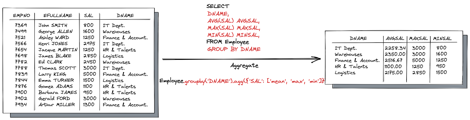
- Aggregating: provides data summaries or statistics such as averages and sums. These calculations are done on multiple values to return a single result. However, the count function considers NULL values when performing its calculation;
- Derivation: which is cross-column calculations. A derived field is a column whose value is derived from the value of one or more columns. The value is determined by a formula that can use constant values or values in other columns in the same table field row;

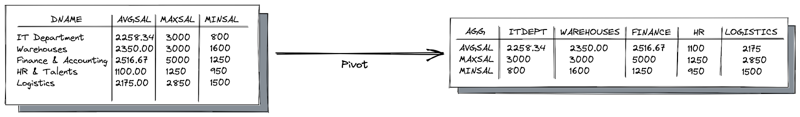
- Pivoting: which involves converting columns values into rows and vice versa. You can use the PIVOT and UNPIVOT relational operators to change a table-valued expression into another table. PIVOT rotates a table-valued expression by turning the unique values from one column in the expression into multiple columns in the output. And PIVOT runs aggregations where they’re required on any remaining column values that are wanted in the final output. UNPIVOT carries out the opposite operation to PIVOT by rotating columns of a table-valued expression into column values;
- Sorting: ordering and indexing of data to enhance search performance. Sorting data is a useful technique for making sense of research information. It helps to organize the raw figures into an understandable form, allowing them to be analyzed and visualized more easily. This can involve sorting all records in their original state or creating aggregated tables, charts, or other summarized outputs. In either case, this process makes interpreting what the data is conveying easier;

- Scaling: normalization and standardization that helps compare different numbers by putting them on a consistent scale. Feature scaling is an essential step in data preprocessing for machine learning. Without it, algorithms that rely on distance measures between features may be biased towards numerically larger values and produce inaccurate results. Scaling helps to ensure all features are given equal weight when computing distances or performing other calculations. Normalization and standardization help compare different numbers by putting them on a consistent scale.
Normalization or Min-Max Scaling is used to transform features on a similar scale. For example, this scales the range to [0, 1] or sometimes [-1, 1]. Normalization is useful when no outliers exist, as it cannot cope with them. For example, we would scale age and not income because only a few people have high incomes, but the age is nearly uniform.
Standardization or Z-Score Normalization transforms features by subtracting from the mean and dividing by standard deviation. This is often called a Z-score. Standardization can be helpful in cases where the data follows a Gaussian distribution. However, this does not have to be necessarily true. Geometrically speaking, it translates the data to the mean vector of the original data to the origin and squishes or expands the points if the standard deviation is 1, respectively. Outliers do not affect standardization because no predefined range of transformed features exists.

- Structure normalization is the process of organizing data into a logical structure that can be used to improve performance and reduce redundancy. This involves breaking down complex datasets into smaller, more manageable pieces by eliminating redundant information or consolidating related items. Normalization also helps ensure consistency in storing and accessing data across different systems. Data denormalizing is the opposite of normalizing; it takes normalized data structures and combines them back together so they are easier to query or analyze as one unit;
- Denormalization is the inverse process of normalization, where the normalized schema is converted into a schema with redundant information. Denormalized data often contain duplicate values that increase storage requirements but make querying faster since all relevant information for a given task may be found within one table instead of having to join multiple tables together first before running queries on them;

Structure Normalization is used in OLTP systems to make insert, delete, and update operations faster. On the other hand, denormalization is used in OLAP systems to optimize search and analysis speed. Normalization ensures data integrity by eliminating redundant data, while denormalizing makes it harder to retain this integrity as more redundant information may be stored. Furthermore, normalization increases the number of tables and joins, whereas denormalizing reduces them. Disk space optimization also differs between these two processes, with normalized tables using less storage than their denormalized counterparts due to duplicate records being eliminated.
- Vectorization: which helps convert non-numerical data into number arrays that are often used for machine learning applications;
- And much more…
4 - Data Modeling
Data modeling has been a practice for decades in one form or another. Since the early 1990s, various normalization techniques have been used to model data in RDBMSs and data warehouses. Data modeling became unfashionable in the early to mid-2010s - The rise of data lake 1.0, NoSQL, and big data platforms allowed engineers to bypass traditional data modeling, sometimes for legitimate performance gains. However, the lack of rigorous data modeling created data swamps, along with lots of redundant, mismatched, or simply wrong data. Nowadays, we don’t talk about “big data”; we instead prefer the term “useful data” and the clockwise swinging back toward rigorously modeled data (e.g., data lakehouse).
A data model depicts the relationship between data and the real world. It outlines the optimal way to structure and standardize data to accurately reflect your organization’s processes, definitions, workflows, and logic. When modeling data, it’s essential to concentrate on translating the model into tangible business outcomes. An effective data model should align with significant business decisions. The process of data modeling involves transitioning from abstract modeling concepts to concrete implementation. This continuum comprises three primary data models: conceptual, logical, and physical.
- Conceptual model: a data model that represents high-level or abstract concepts and relationships between them in a simplified manner (ER diagrams). It serves as a starting point for developing more detailed models. In addition, it provides a big-picture view (business logic and rules) of the data and its relationships to the organization’s business processes. A conceptual model focuses on the overall structure and meaning of the data rather than specific technical details or implementation considerations. It is often used in the early stages of the data modeling process to facilitate communication between different stakeholders, including business analysts, subject matter experts, and technical teams.
- Logical model: a logical data model is a type of data model that provides a detailed representation of the data and its relationships to the business processes of an organization. It is a more detailed and refined version of a conceptual data model and provides a bridge between the high-level business view and the technical implementation. It focuses on the data structure, including tables, columns, keys, and indexes, while avoiding any technical implementation details. It serves as a blueprint for designing the physical data model, which is used to implement the data model in a specific database management system.
- Physical model: defines how the logical model will be implemented in a data storage technology.

You should generally strive to model your data at the finest grain possible. From here, it’s easy to aggregate this highly granular dataset. Unfortunately, the reverse isn’t true, and restoring details that have been aggregated away is generally impossible. This is where data normalization comes into the picture.
The practice of normalization in data modeling involves implementing strict control over the relationships of tables and columns within a database to eliminate data redundancy and ensure referential integrity. This concept was initially introduced by Edgar Codd, a pioneer in relational databases, in the early 1970s through the introduction of normal forms. The normal forms are hierarchical in nature, with each subsequent form building upon the requirements of the previous one. Here are Codd’s first three normal forms:
- First normal form (1NF): The table must have a primary key, and each column in the table should contain atomic values (i.e., indivisible values);
- Second normal form (2NF): The table must already be in the first normal form, and all non-key attributes must fully depend on the primary key;
- Third normal form (3NF): The table must already be in the second normal form, and all non-key attributes should be dependent on the primary key only and not on other non-key attributes.
There are also additional normal forms beyond 3NF, such as the Boyce-Codd Normal Form (BCNF), Fourth Normal Form (4NF), and Fifth Normal Form (5NF), which build on the principles of the earlier normal forms to further reduce data redundancy and improve data integrity. Here are brief explanations of each:
- Boyce-Codd Normal Form (BCNF): Also known as 3.5NF, this normal form is an extension of 3NF that requires that every determinant (attribute or set of attributes that uniquely determines another attribute) in a table is a candidate key. This eliminates some types of anomalies that can still occur in 3NF tables.
- Fourth Normal Form (4NF): A table is in 4NF if it has no multi-valued dependencies. A multi-valued dependency occurs when a table has attributes that are dependent on only part of a multi-valued key. Data redundancy can be reduced by separating such attributes into a separate table.
- Fifth Normal Form (5NF): Also known as Project-Join Normal Form (PJNF), this normal form deals with the issue of join dependencies, which occur when a table can be reconstructed by joining multiple smaller tables. Tables in 5NF have no join dependencies, meaning they cannot be further decomposed into smaller tables without losing information.

When describing data modeling for data lakes or data warehouses, you should assume that the raw data takes many forms (e.g., structured and semistructured). Still, the output is a structured data model of rows and columns. However, several approaches to data modeling can be used in these environments. You’ll likely encounter the following famous methods: Kimball, Inmon, and Data Vault.
In practice, some of these techniques can be combined. For example, some data teams start with Data Vault and then add a Kimball star schema alongside it.
Inmon’s data modeling
Inmon defines a data warehouse: “A data warehouse is a subject-oriented, integrated, nonvolatile, and time-variant collection of data in support of management’s decisions. The data warehouse contains granular corporate data. Data in the data warehouse can be used for many different purposes, including sitting and waiting for future requirements which are unknown today.”
The four critical characteristics of a data warehouse can be described as follows:
- Subject-oriented: The data warehouse focuses on a specific subject area, such as sales or accounting;
- Integrated: Data from disparate sources is consolidated and normalized;
- Nonvolatile: Data remains unchanged after it is stored in a data warehouse;
- Time-variant: Varying time ranges can be queried.
To create a logical model, the first step is to focus on a specific area. For example, if the area of interest is “sales,” then the logical model should encompass all the relevant details related to sales, such as business keys, relationships, and attributes. Next, these details are consolidated and integrated into a highly normalized data model. The strict normalization requirement ensures as little data duplication as possible, which leads to fewer downstream analytical errors because data won’t diverge or suffer from redundancies.
The data warehouse represents a “single source of truth,” which supports the overall business’s information requirements. The data is presented for downstream reports and analysis via business and department-specific data marts, which may also be denormalized. Finally, the data is stored in a nonvolatile and time-variant manner, meaning you can (theoretically) query the original data for as long as storage history allows.
Kimball Star Schema
A popular option for modeling data in a data mart is a star schema (Kimball), though any data model that provides easily accessible information is also suitable. Created by Ralph Kimball in the early 1990s, this approach to data modeling focuses less on normalization and, in some cases accepting denormalization.
In contrast to Inmon’s approach of integrating data from across the business into the data warehouse and then providing department-specific analytics via data marts, the Kimball model is bottom-up and promotes modeling and serving department or business analytics directly within the data warehouse. Inmon argues that this approach distorts the definition of a data warehouse: By making the data mart the data warehouse itself, the Kimball approach allows for faster iteration and modeling than Inmon, but this comes at the cost of potentially looser data integration, data redundancy, and duplication.
In Kimball’s approach, data is modeled with two general types of tables: facts and dimensions. You can think of a fact table as a table of numbers and dimension tables as qualitative data referencing a fact. Dimension tables surround a single fact table in a relationship called a star schema:
- Fact tables contain factual, quantitative, and event-related data. The data in a fact table is immutable because facts relate to events. Therefore, fact tables don’t change and are append-only. Fact tables are typically narrow and long, meaning they don’t have many columns but many rows representing events. Fact tables should be at the finest grain possible.
- Dimension tables provide the reference data, attributes, and relational context for the events stored in fact tables. Dimension tables are smaller than fact tables, typically wide and short, and take an opposite shape. When joined to a fact table, dimensions can describe the events’ what, where, and when. Dimensions are denormalized1, with the possibility of duplicate data (allowed in the Kimball data model).
- Slowly changing dimensions (SCD) refers to specific kinds of dimension tables typically used to track changes in dimensions over time. There exist seven types of SCD:
- Type 0: This type of SCD doesn’t track changes to a dimension at all. In other words, the dimension is treated as static, and the data never changes. This is useful when the dimension is a constant and doesn’t change over time.
- SCD Type 1: This approach overwrites the existing data with the new data. In other words, the dimension record is updated in place with the new information, and the old data is lost. This method is useful when historical data isn’t important or when the data volume is small.
- SCD Type 2: This type of SCD creates a new record every time a change is made to a dimension. In other words, the historical data is preserved by adding a new row to the table with a new primary key value. Each record has a start and end date, so you can track the changes over time. This method is useful when historical data is important, and you need to be able to analyze the changes over time.
- SCD Type 3: This approach adds a new column to an existing record to track a change in a dimension. In other words, the old value is preserved in the original column, while the new value is stored in a new column. This method is useful when you need to track only a few changes to a dimension over time.
- SCD Type 4: Overwrite existing dimension records, just like SCD Type 1. However, we simultaneously maintain a history table to keep track of these changes. This method is useful when the dimension table is large, and storing historical data in the same table could cause performance issues.
- SCD Type 5: This approach combines the Type 1 and Type 2 SCDs. In other words, it updates the existing record with the new data, but it also creates a new record to track the history. This method is useful when you need to keep both current and historical data and you also need to track changes over time.
- SCD Type 6: This type of SCD combines Type 2 and Type 3 SCDs. In other words, it stores the history of changes in separate columns, similar to Type 3 SCD, but it also creates a new record for each change, similar to Type 2 SCD. This method is useful when you need to track specific changes to a dimension over time while preserving the old and new data.
- SCD Type 7 is a relatively new approach to Slowly Changing Dimensions and is sometimes called the “Hybrid SCD.” It combines the Type 1 and Type 2 SCDs with the addition of a “Current Flag” column in the dimension table. The “Current Flag” column indicates which row represents the current version of the dimension. This flag is set to “Y” for the current version and “N” for all other historical versions. This method provides a balance between preserving historical data (like Type 2 SCD) and maintaining simplicity (like Type 1 SCD). It also simplifies querying for the current and historical versions of the dimension and reduces the number of joins required to access the data.
- Star schema represents the data model of the business. Unlike highly normalized approaches to data modeling, the star schema is a fact table surrounded by the necessary dimensions. This results in fewer joins than other data models, which speeds up query performance. Another advantage of a star schema is it’s arguably more accessible for business users to understand and use.

Because a star schema has one fact table, sometimes you’ll have multiple star schemas that address different business facts. For example, sales, marketing, and purchasing can have their own star schema fed upstream from the granular data in the data warehouse. This allows each department to have a unique and optimized data structure for its specific needs.
You should strive to reduce the number of dimensions whenever possible since this reference data can potentially be reused among different fact tables. A dimension that is reused across multiple star schemas, thus sharing the same fields is called a conformed dimension. A conformed dimension allows you to combine multiple fact tables across multiple star schemas.
Data vault
Whereas Kimball and Inmon focus on the structure of business logic in the data warehouse, the Data Vault offers a different approach to data modeling. Created in the 1990s by Dan Linstedt, the Data Vault methodology separates the structural aspects of a source system’s data from its attributes. Instead of representing business logic in facts, dimensions, or highly normalized tables, a Data Vault simply loads data from source systems directly into a handful of purpose-built tables in an insert-only manner. Unlike the other data modeling approaches you’ve learned about, there’s no notion of good, bad, or conformed data in a Data Vault.
A Data Vault model consists of three main tables: hubs, links, and satellites. In short, a hub stores business keys, a link maintains relationships among business keys, and a satellite represents a business key’s attributes and context. A user will query a hub that links to a satellite table containing the query’s relevant attributes.
- Hubs: Queries often involve searching by a business key, such as a customer ID or an order ID from our e-commerce example. A hub is the central entity of a Data Vault that retains a record of all unique business keys loaded into the Data Vault. A hub always contains the following standard fields:
- Hash key: The primary key used to join data between systems. This is a calculated hash field (MD5 or similar);
- Load date: The date the data was loaded into the hub;
- Record source: The source from which the unique record was obtained;
- Business key(s): The key used to identify a unique record.
Note: It’s important to note that a hub is insert-only, and data is not altered in a hub. Once data is loaded into a hub, it’s permanent.
- Link tables track the relationships of business keys between hubs. Link tables connect hubs, ideally at the lowest possible grain. Because link tables connect data from various hubs, they are many to many. The Data Vault model’s relationships are straightforward and handled through changes to the links. This provides excellent flexibility in the inevitable event that the underlying data changes. You simply create a new link that ties business concepts (or hubs) to represent the new relationship.
- Satellites: We’ve described relationships between hubs and links that involve keys, load dates, and record sources. How do you get a sense of what these relationships mean? Satellites are descriptive attributes that give meaning and context to hubs. Satellites can connect to either hubs or links. The only required fields in a satellite are a primary key consisting of the business key of the parent hub and a load date. Beyond that, a satellite can contain however many attributes that make sense.

Other types of Data Vault tables exist, including point-in-time (PIT) and bridge tables. However, I won’t cover these here since my goal is to simply give you an overview of the Data Vault’s power.
Unlike other data modeling techniques we’ve discussed, the business logic is created and interpreted in a Data Vault when the data from these tables are queried. Please be aware that the Data Vault model can be used with other data modeling techniques. For example, it’s not unusual for a Data Vault to be the landing zone for analytical data. After that, it’s separately modeled in a data warehouse, commonly using a star schema. The Data Vault model also can be adapted for NoSQL and streaming data sources.
5 - Data Lineage
Keeping track of the relationships between and within datasets is increasingly important as data sources are added, modified, or updated. This can range from a simple column renaming to complex joins across multiple tables sourced from different databases that may have undergone several transformations. Lineage provides traceability for understanding where fields and datasets come from and an audit trail for tracking when changes were made, why they were made, and by whom. Even with purpose-built solutions, capturing all this information in a Data Lake environment takes time and effort. Lineage requires aggregating logs at both transactional (who accessed what) and structural/filesystem levels (relationships between datasets). It involves any batch processing tools such as MapReduce or Spark but also external systems like RDBMSs that manipulate the data.

Tracking data lineage is essential to ensure that strategic decisions are based on accurate information. Without it, verifying the source and transformation of data can be costly and time-consuming. Data lineage helps users confirm that their data has been sourced from a reliable source, transformed correctly, and loaded into the intended destination.
Here are a few common techniques used to perform data lineage on strategic datasets:
Pattern-Based Lineage
This technique uses metadata to trace the data lineage without analyzing the pipeline implementation. It looks for patterns in tables, columns, and business reports by comparing similar names and values between datasets. These two elements are linked on a data lineage chart to show how they relate if a match is found. This method can be used to quickly identify relationships between different stages of the same dataset’s lifecycle.
The primary benefit of pattern-based lineage is its versatility; it does not rely on any specific technology and can be used across different databases, such as Oracle and MySQL. However, this approach may lack accuracy since connections between datasets could potentially go undetected if the data processing logic is hidden in pipeline implementation rather than being visible in human-readable metadata.
Lineage by Data Tagging
This technique relies on the tags that transformation engines add to the processed data. By tracking these tags from start to finish, it is possible to discover lineage information about the data. However, for this method to be effective, there must be consistent usage of the same transformation tool across all data movements and an understanding of its tagging structure. Furthermore, since external sources generated outside this system are not tagged by default, they cannot benefit from such lineage tracing via tagging alone; thus making it suitable only for closed systems without external sources.
Self-Contained Lineage
Some organizations have a sole data environment that provides storage, processing logic, and master data management (MDM) for central control over metadata. This self-contained system can inherently provide lineage without the need for external tools. However, it will be unaware of any changes or updates made outside this controlled environment.
Lineage by Parsing (reverse engineering)
This is the most advanced form of lineage. It automatically reads the logic used to process data to trace data transformation from end to end. Capturing changes across systems is easy with this form of data lineage since it tracks data as it moves. However, it requires a high understanding of the programming languages or tools used throughout the data lifecycle. To deploy this solution, one must understand all programming languages and tools used for transforming and moving the data, such as ETL tools, SQL queries, and programming languages used to create pipelines. This can be a complex process, but it provides comprehensive tracing capabilities.
Lineage using Data Contracts
As seen in the Data cleaning section, Data Contracts hold information about schema and semantics, both versioning and the SLA agreements between producers and consumers. Moreover, data contracts can also contain detailed information about lineage, like tags, data owners, data sources, Intended Consumers, etc.
Data Processing Underlying Activities
In the processing stage, your data mutates and morphs into something useful for the business. Because there are many moving parts, the underlying activities are especially critical at this stage.
- Security: Access to specific columns, rows, and cells within a dataset should also be controlled. It’s crucial to be mindful of potential attack vectors against your database during query time. You must tightly monitor, and control read/write privileges to the database. Query access to the database should be controlled in the same manner as access to your organization’s systems and environments. To ensure security, credentials such as passwords and access tokens should be kept hidden and never copied and pasted into code or unencrypted files.
- Data Management: To ensure data accuracy during transformations, it’s crucial to ensure that the data used is defect-free and represents the ground truth. Implementing Master Data Management (MDM) at your company can be a viable option to achieve this goal. MDM plays a significant role in preserving the original integrity and ground truth of data, which is essential for conformed dimensions and other transformations. If implementing MDM is not possible, working with upstream stakeholders who control the data can help ensure that the transformed data is accurate and complies with the agreed-upon business logic.
- DataOps: queries and transformations require monitoring and alerting in two key areas: data and systems. Changes or anomalies in these areas must be promptly detected and addressed. The field of data observability is rapidly expanding, with a strong emphasis on data reliability. Recently, a new job title called “data reliability engineer” has emerged, highlighting the importance of ensuring data reliability. Data observability and health are critical components in this context, particularly during the query and transformation stages. By emphasizing these areas, DataOps can ensure that data is reliable and the systems that process it are functioning optimally.
- Orchestration: Data teams often manage their transformation pipelines using simple time-based schedules (e.g., cron jobs). This works reasonably well initially but becomes a nightmare as workflows become more complicated. Instead, use orchestration to manage complex pipelines using a dependency-based approach. Orchestration is also the glue that allows us to assemble pipelines that span multiple systems.
- Data architecture: as I highlighted in Data 101 - part 3, about what makes a good data architecture, I explained that a good data architecture should primarily serve business requirements with a widely reusable set of building blocks while preserving well-defined best practices (principles) and making appropriate trade-offs. When designing a processing system for your data journey, you must be aware of your business constraints, challenges, and how your data initiative will evolve. You can assess your architecture against the six pillars of AWS Well-Architected Framework (WAF):
- Operational excellence: You must adopt approaches that improve change flows into production, that enable refactoring, provide fast feedback on quality, and bug fixing. These accelerate beneficial changes entering production, limit issues deployed, and enable rapid identification and remediation of issues introduced through deployment activities. In addition, evaluate the operational readiness of your data processing workloads, and understand the operational risks related to these ones.
- Security: Compute resources used in your processing workloads require multiple layers of defense to help protect from external and internal threats. Enforcing boundary protection, monitoring points of ingress and egress, and comprehensive logging, monitoring, and alerting are all essential to an effective information security plan.
- Reliability: Build highly scalable and reliable workloads using a domain-driven design (DDD). Adopting a data product approach makes transformation smaller, simpler, and reusable. In addition, most querying and transformation workloads are distributed (e.g., MapReduce) and thus rely on communications networks to interconnect workloads workers. Your workload must operate reliably despite data loss or latency in these networks. Components of the distributed system must operate in a way that does not negatively impact other components or the workload. These best practices prevent failures and improve the mean time between failures (MTBF) and the mean time to recovery (MTTR).
- Performance efficiency: The optimal compute solution for a workload varies based on your data product and business constraints. Data Architectures must carefully choose different compute solutions for various workloads and enable different features to improve performance. Selecting the wrong compute solution for an architecture can lead to lower performance efficiency.
- Cost optimization: You should monitor and manage compute usage and costs and Implement change control and resource management from project inception to end-of-life. This ensures you shut down or terminate unused resources to reduce waste.
- Sustainability: To minimize the environmental impacts of running the data processing workloads, you must implement Implement patterns for performing load smoothing and maintaining consistent high utilization of deployed resources to reduce the resources required to support your workload and the resources needed to use it.
Summary
Transformations are a crucial aspect of data pipelines, as they lie at the heart of the process. However, it’s essential to always keep in mind the purpose of these transformations. Engineers are not hired simply to experiment with the latest technological toys but to serve their customers. In this process, data is converted and structured from a particular form into a usable form that adds value and return on investment (ROI) to the business.
In this post, we’ve seen more details about data processing and what it consists of. The data processing step starts with data cleansing (pre-processing), which makes data reliable, and lasts with data modeling that depicts the relationship between data and the real world. A tremendous universe of tools, solutions, and principles is implemented between these two steps to gain insights and support decision-making processes.
As we head into the data journey’s serving stage (in the next post), it’s important to reflect on technology as a tool for achieving organizational goals. If you’re currently working as a data engineer, consider how improvements in transformation systems could enhance your ability to serve end customers better. This may involve using new tools, technologies, or processes to extract more value from data and make it more accessible to end users. On the other hand, if you’re just starting on a path toward data engineering, consider the business problems that interest you and how technology can be leveraged to solve them. You can create data-driven solutions that deliver value to your customers and your organization by identifying your industry’s specific challenges and opportunities. Ultimately, technology should always be viewed as a means to an end, and the key to successful data engineering is using it to serve your broader business objectives.
References
- H. W. Inmon, Building the Data Warehouse (Hoboken: Wiley, 2005).
- Ackerman H., King J., Operationalizing the Data Lake (O’Reilly Media 2019).
- Daniel Linstedt and Michael Olschimke, Building a Scalable Data Warehouse with Data Vault 2.0 (Morgan Kaufmann).
- “Data Vault 2.0 Modeling Basics”, Kent Graziano (Snowflake).
- “Data Warehouse: The Choice of Inmon versus Kimball”, Ian Abramson.
- “What is Data Lineage?”, Imperva Blog.
- “Introduction to Secure Data Sharing”, Snowflake docs.
- “Qu’est-ce que Data as a Service (DaaS) ?”, Tibco.
- “Augmented Data Catalogs: Now an Enterprise Must-Have for Data and Analytics Leaders”, Ehtisham Zaidi, and Guido De Simoni (Gartner).
- “Data preparation – its applications and how it works”, Talend Resources.
- “Data Discovery: A Closer Look at One of 2017’s Most Important BI Trends”, BARC.
- “Cleaning Big Data: Most Time-Consuming, Least Enjoyable Data Science Task, Survey Says”, Gil Press (Forbes).
- “Guide To Data Cleaning: Definition, Benefits, Components, And How To Clean Your Data”, Tableau Blog.
- “The Rise of Data Contracts And Why Your Data Pipelines Don’t Scale”, Chad Sanderson.
- “Comparison of different file formats in Big Data”, Aida NGOM (Adatlas).
- You can preserve dimensions normalization with “Snowflaking”. The principle behind snowflaking is the normalization of the dimension tables by removing low cardinality attributes and forming separate tables. The resultant structure resembles a snowflake with the fact table in the middle.