
Data processing is at the core of any data architecture. It involves transforming raw data into useful insights through analysis techniques like machine learning algorithms or statistical models depending on what type of problem needs solving within an organization’s context.
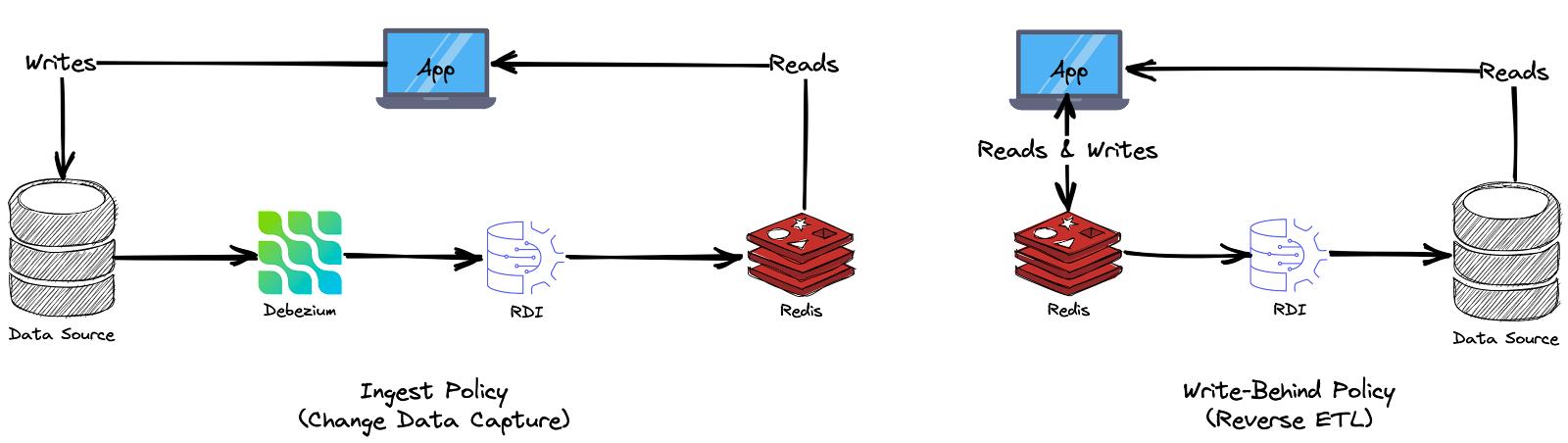
We have seen in the past posts that raw data, already extracted from data sources, can be prepared and transformed (using Redis Gears) into the target format required by the downstream systems. In this post, we push this concept further by coupling the event-processing of RedisGears and stream-based ingestion using Redis Data Integration (RDI). Thus, you can imagine that data flowing in your operational systems (e.g., ERPs, CRMs…) will be ingested into Redis using a Change Data Capture (see Data & Redis - part 1) and processed with RedisGears to derive rapid operational decisions in near real-time.
In fact, Redis Data Integration is not only a data integration tool but also a data processing engine that relies on Redis Gears. Therefore, it provides a more straightforward way to implement data transformations (declarative files) to avoid the complexity of Redis Gears.
Pre-requisites
1 - Create a Redis Database
For this article, you need to install and set up a few things. First, you need to prepare a Redis Enterprise Cluster, which is the target storage support. This storage support will be the target infrastructure for the data transformed in this stage. You can use this project to create a Redis Enterprise cluster in the cloud provider of your choice.
Once you have created a Redis Enterprise cluster, you must create a target database that holds the transformed data. Redis Enterprise Software lets you create and distribute databases across a cluster of nodes. To create a new database, follow the instructions here.
For Redis Data Integration, you need two databases: the config database exposed on redis-12000.cluster.redis-process.demo.redislabs.com:12000 and the target database on: redis-13000.cluster.redis-process.demo.redislabs.com:13000. Don’t forget to add the RedisJSON module when you create the target database.
2 - Install RedisGears
Now, let’s install RedisGears on the cluster. In case it’s missing, follow this guide to install it.
curl -s https://redismodules.s3.amazonaws.com/redisgears/redisgears.Linux-ubuntu20.04-x86_64.1.2.5.zip -o /tmp/redis-gears.zip
curl -v -k -s -u "<REDIS_CLUSTER_USER>:<REDIS_CLUSTER_PASSWORD>" -F "module=@/tmp/redis-gears.zip" https://<REDIS_CLUSTER_HOST>:9443/v2/modules
3 - Install Redis Data Integration (RDI)
For the second part of this article, you will need to install Redis Data Integration (RDI). Redis Data Integration installation is done via the RDI CLI. The CLI should have network access to the Redis Enterprise cluster API (port 9443 by default). You need first to download the RDI offline package:
UBUNTU20.04
wget https://qa-onprem.s3.amazonaws.com/redis-di/latest/redis-di-offline-ubuntu20.04-latest.tar.gz -O /tmp/redis-di-offline.tar.gz
UBUNTU18.04
wget https://qa-onprem.s3.amazonaws.com/redis-di/latest/redis-di-offline-ubuntu18.04-latest.tar.gz -O /tmp/redis-di-offline.tar.gz
RHEL8
wget https://qa-onprem.s3.amazonaws.com/redis-di/latest/redis-di-offline-rhel8-latest.tar.gz -O /tmp/redis-di-offline.tar.gz
RHEL7
wget https://qa-onprem.s3.amazonaws.com/redis-di/latest/redis-di-offline-rhel7-latest.tar.gz -O /tmp/redis-di-offline.tar.gz
Then Copy and unpack the downloaded redis-di-offline.tar.gz into the master node of your Redis Cluster under the /tmp directory:
tar xvf /tmp/redis-di-offline.tar.gz -C /tmp
Then you install the RDI CLI by unpacking redis-di.tar.gz into /usr/local/bin/ directory:
sudo tar xvf /tmp/redis-di-offline/redis-di-cli/redis-di.tar.gz -C /usr/local/bin/
Run create command to set up the Redis Data Integration config database (on port 13000) instance within an existing Redis Enterprise Cluster:
redis-di create --silent --cluster-host <CLUSTER_HOST> --cluster-user <CLUSTER_USER> --cluster-password <CLUSTER_PASSWORD> --rdi-port <RDI_PORT> --rdi-password <RDI_PASSWORD> --rdi-memory 512
Finally, run the scaffold command to generate configuration files for Redis Data Integration and Debezium Redis Sink Connector:
redis-di scaffold --db-type <cassandra|mysql|oracle|postgresql|sqlserver> --dir <PATH_TO_DIR>
In our article, we will capture a SQL Server database, so choose (sqlserver). The following files will be created in the provided directory:
├── debezium
│   └── application.properties
├── jobs
│   └── README.md
└── config.yaml
config.yaml- Redis Data Integration configuration file (definitions of target database, applier, etc.)debezium/application.properties- Debezium Server configuration filejobs- Data transformation jobs, read here
To use debezium as a docker container, download the debezium Image
wget https://qa-onprem.s3.amazonaws.com/redis-di/debezium/debezium_server_2.1.1.Final_offline.tar.gz -O /tmp/debezium_server.tar.gz
and load it as a docker image.
docker load < /tmp/debezium_server.tar.gz
Then tag the image:
docker tag debezium/server:2.1.1.Final_offline debezium/server:2.1.1.Final
docker tag debezium/server:2.1.1.Final_offline debezium/server:latest
For the non-containerized deployment, you need to install Java 11 or Java 17. Then download Debezium Server 2.1.1.Final from here.
Unpack Debezium Server:
tar xvfz debezium-server-dist-2.1.1.Final.tar.gz
Copy the scaffolded application.properties file (created by the scaffold command) to the extracted debezium-server/conf directory. Verify that you’ve configured this file based on these instructions.
If you use Oracle as your source DB, please note that Debezium Server does not include the Oracle JDBC driver. You should download it and locate it under the debezium-server/lib directory:
cd debezium-server/lib
wget https://repo1.maven.org/maven2/com/oracle/database/jdbc/ojdbc8/21.1.0.0/ojdbc8-21.1.0.0.jar
Then, start Debezium Server from the debezium-server directory:
./run.sh
Data processing using Redis Data Integration
Data transformation is a critical part of the data journey. This process can perform constructive tasks such as adding or copying records and fields, destructive actions like filtering and deleting specific values, aesthetic adjustments to standardize values, or structural changes that include renaming columns, moving them around, and merging them together.
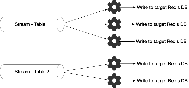
The key functionality offered by RDI is mapping the data coming from Debezium Server (representing a Source Database row data or row state change) into a Redis key/value pair. The incoming data includes the schema. By default, each source row is converted into one Hash or one JSON key in Redis. RDI will use a set of handlers to automatically convert each source column to a Redis Hash field or a JSON attribute based on the Debezium type in the schema.
However, if you want to customize this default mapping or add a new transformation, RDI provides Declarative Data Transformations (YAML files). Each YAML file contains a Job, a set of transformations per source table. The source is typically a database table or collection and is specified as the full name of this table/collection. The job contains logical steps to transform data into the desired output and store it in Redis (as Hash or JSON). All of these files will be uploaded to Redis Data Integration using the deploy command when they are available under the jobs folder:
├── debezium
│   └── application.properties
├── jobs
│   └── README.md
└── config.yaml
We’ve seen in Data 101 - part 5 that the pipelines required to run the transformation processes can be implemented using one of these approaches:
- Code-centric tools: analysis and manipulation libraries built on top of general-purpose programming languages (Scala, Java or Python). These libraries manipulate data using the native data structures of the programming language.
- Query-centric tools: use a querying language like SQL (Structured Query Language) to manage and manipulate datasets. These languages can be used to create, update and delete records, as well as query the data for specific information.
- Hybrid tools: implement SQL on top of general-purpose programming languages. This is the case for libraries like Apache Spark or Apache Kafka, which provides a SQL dialect called KSQL.
Redis Data Integration (RDI) leverages the hybrid approach since all transformation jobs are implemented using a human-readable format (YAML files) that embeds JMESPath and/or SQL.

The YAML files accept the following blocks/fields:
source - This section describes what is the table that this job works on:
server_name: logical server name (optional)db: DB name (optional)schema: DB schema (optional)table: DB tablerow_format: Format of the data to be transformed: data_only (default) - only payload, full - complete change record
transform: his section includes a series of blocks that the data should go through. See documentation of the supported blocks and JMESPath custom functions.
output - This section includes the outputs where the data should be written to:
- Redis:
uses:redis.write: Write to a Redis data structure
with:connection: Connection namekey: This allows to override the key of the record by applying a custom logic:expression: Expression to executelanguage: Expression language, JMESPath, or SQL
- SQL:
uses:relational.write: Write into a SQL-compatible data store
with:connection: Connection nameschema: Schematable: Target tablekeys: Array of key columnsmapping: Array of mapping columnsopcode_field: Name of the field in the payload that holds the operation (c - create, d - delete, u - update) for this record in the DB
I’ve detailed many data transformations archetypes in Data 101 - part 5 and find it interesting to evaluate Redis Data Integration through this list of capabilities. Thus, you can see how to perform different kinds of transformations using RDI.
1 - Filtering
This process selects a subset from your dataset (specific columns) that require transformation, viewing, or analysis. This selection can be based on certain criteria, such as specific values in one or more columns, and it typically results in only part of the original data being used. As a result, filtering allows you to quickly identify trends and patterns within your dataset that may not have been visible before. It also lets you focus on particular aspects of interest without sifting through all available information. In addition, this technique can reduce complexity by eliminating unnecessary details while still preserving important insights about the underlying data structure.

Using Redis Data Integration, filtering the Employee’s data (example above) to keep only people having a salary that exceeds 1,000 can be implemented using the following YAML blocks:
source:
  table: Employee
transform:
  - uses: filter
    with:
      language: sql
      expression: SAL>1000
When you put this YAML file under the jobs folder, Redis Data Integration will capture changes from the source table and apply the filter to store only records confirming the filtering expression (see Data & Redis - part 1 for RDI and SQL Server configuration).

2 - Enriching
This process fills out the basic gaps in the data set. It also enhances existing information by supplementing incomplete or missing data with relevant context. It aims to improve accuracy, quality, and value for better results.
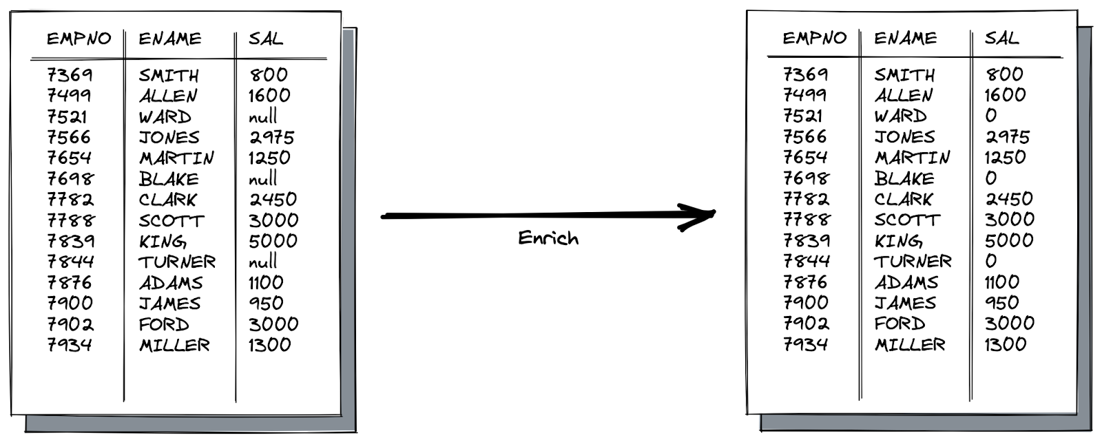
Let’s assume the example above. We need to replace all NULL salaries in the Employee’s table with a default value of 0. In SQL, the COALESCE function returns the first non-NULL value in the attribute list. Thus COALESCE(SAL, 0) returns the salary if it is not null or 0 elsewhere. With RDI, we can implement this enrichment using the following job:
source:
    table: Employee
  transform:
    - uses: map
      with:
        expression:
          EMPNO: EMPNO
          ENAME: ENAME
          SAL: COALESCE(SAL, 0)
        language: sql
In this configuration, we used the map block that maps each source record into a new output based on the expressions. Here we changed only the salary field that implements the COALESCE expression.

If you are using SQL Server, another alternative to performing this enrichment is to use the ISNULL function. Thus, we can use ISNULL(SAL, 0) in the expression block. The ISNULL function and the COALESCE expression have a similar purpose but can behave differently. Because ISNULL is a function, it is evaluated only once. However, the input values for the COALESCE expression can be evaluated multiple times. Moreover, the data type determination of the resulting expression is different. ISNULL uses the data type of the first parameter, COALESCE follows the CASE expression rules and returns the data type of value with the highest precedence.
source:
  table: Employee
transform:
  - uses: map
    with:
      expression:
        EMPNO: EMPNO
        ENAME: ENAME
        SAL: ISNULL(SAL, 0)
      language: sql
3 - Splitting
Splitting fields into multiple ones consists of two atomic operations: adding the new fields according to specific transformation rules, then removing the source field (split column).

In the example above, we split the EFULLNAME into two fields: ELASTNAME and EFIRSTNAME. The following configuration uses the add_field block to create the new fields ELASTNAME and EFIRSTNAME. Then, we can use the SUBSTRING function from SQL or the SPLIT function from JMESPath. In both cases, we need the additional block remove_field to remove the source column EFULLNAME.
source:
  table: Employee
transform:
  - uses: add_field
    with:
      fields:
        - field: EFIRSTNAME
          language: jmespath
          expression: split(EFULLNAME, ', ')[0]
        - field: ELASTNAME
          language: jmespath
          expression: split(EFULLNAME, ', ')[1]
  - uses: remove_field
    with:
      field: EFULLNAME
The split function breaks down the EFULLNAME into an array using the string separators provided as parameters (the comma character as separator).

4 - Merging
Merging multiple fields into one consists of two atomic operations: adding the new field according to a specific transformation rule, then removing the source fields (merged columns).

In the example above, we merge the EFIRSTNAME and ELASTNAME into one field: EFULLNAME. The following configuration uses the add_field block to create the new fields EFULLNAME and two remove_field blocks to remove the merged columns EFIRSTNAME and ELASTNAME. To express the transformation rule, we can use the CONCAT_WS function from SQL or the JOIN / CONCAT functions from JMESPath.
source:
  table: Employee
transform:
  - uses: add_field
    with:
      fields:
        - field: EFULLNAME
          language: jmespath
          expression: concat([EFIRSTNAME, ' ', ELASTNAME])

  - uses: remove_field
    with:
      fields:
        - field: EFIRSTNAME
        - field: ELASTNAME

5 - Removing
Besides removing specific columns from the source using the remove_field block or even avoiding the load of some columns using filtering. We might need to drop parts of data according to a specific condition, such as duplicates. In this case, Redis Data Integration doesn’t have a specific block or function to perform the drop of duplicates. However, we can use the key block to create a custom key for the output composed of all fields that form the duplicate.

For example, let’s assume the use case above. If we observe the EMPNO column, we have a distinct ID for each record. However, three records are duplicates, in fact. So, in this case, we want to drop these duplicates according to the EFULLNAME and SAL fields and not to EMPNO. The solution in RDI is to create a new key that preserves the unicity of records: A key composed of the concatenation of EFULLNAME and SAL. Thus RDI can drop any duplicates based on the newly created key.
source:
  table: Employee
output:
  - uses: redis.write
    with:
      connection: target
      key:
        expression: hash(concat([EFULLNAME, '-', SAL]), 'sha3_512')
        language: jmespath
In addition, we use the hash function to create an ID instead of a set of concatenated fields. However, beware that It may be possible that two concatenations (different strings) have the same hash values. This may occur because we take modulo ‘M’ in the final hash value. In that case, two different combinations of (EFULLNAME ‘-‘ SAL) may have the same hash values, called a collision.
However, the chances of random collisions are negligibly small for even billions of assets. Because the SHA-3 series is built to offer 2n/2 collision resistance. In our transformation, we’ve chosen SHA3-512, which offers 2256 (or 1 chance over 115,792,089,237,316,195,423,570,985,008,687,907,853,269,984,665,640,564,039,457,584,007,913,129,639,936 to get another String combination having the same hash!
6 - Derivation
The derivation is cross-column calculations. With RDI, we can easily create a new field based on calculations from existing fields. Let’s assume the example below. We need to calculate the total compensation of each employee based on the salaries and bonuses they get.

The following job implements this kind of derivation using SQL by summing up the SAL and BONUS fields and storing them into one additional field called TOTALCOMP:
source:
  table: Employee
transform:
  - uses: add_field
    with:
      fields:
        - field: TOTALCOMP
          language: sql
          expression: SAL + BONUS
7 - Data Denormalization
Redis Data Integration (RDI) has a different approach to performing joins between two tables that have one-to-many or many-to-one relationships. This approach is called the nesting strategy. It consists of organizing data into a logical structure where the parent-children relationship is converted into a schema based on nesting. Denormalized data often contain duplicate values when represented as tables or hashes, increasing storage requirements but making querying faster since all relevant information for a given task may be found within one table instead of having to join multiple tables/hashes together first before running queries on them.

However, you can choose to perform the denormalization using JSON format. In this case, no duplication will be represented; thus no impact on the storage since the parent-children relationship is just reflected hierarchically.
Let’s assume the two tables: Department and Employee. We will create a declarative data transformation that denormalizes these two tables into one nested structure in JSON. The aim is to get the details of employees in each department.

Let’s create the following file in the jobs directory. This declarative file merges the two tables into a single JSON object. It also demonstrates how easy to set such a complex transformation using a simple YAML declarative file.
source:
  table: Employee
output:
  - uses: redis.write
    with:
      nest:
        parent:
          table: Department
        nesting_key: EMPNO         # cannot be composite
        parent_key: DEPTNO         # cannot be composite
        path: $.Employees          # path must start from root ($)
        structure: map
Using the Debezium SQL Server connector is a good practice to have a dedicated user with the minimal required permissions in SQL Server to control blast radius. For that, you need to run the T-SQL script below:
USE master
GO
CREATE LOGIN dbzuser WITH PASSWORD = 'dbz-password'
GO
USE HR
GO
CREATE USER dbzuser FOR LOGIN dbzuser
GO
And Grant the Required Permissions to the new User
USE HR
GO
EXEC sp_addrolemember N'db_datareader', N'dbzuser'
GO
Then you must enable Change Data Capture (CDC) for each database and table you want to capture.
EXEC msdb.dbo.rds_cdc_enable_db 'HR'
GO
Run this T-SQL script for each table in the database and substitute the table name in @source_name with the names of the tables (Employee and Department):
USE HR
GO
EXEC sys.sp_cdc_enable_table
@source_schema = N'dbo',
@source_name   = N'<Table_Name>',
@role_name     = N'db_cdc',
@supports_net_changes = 0
GO
Finally, the Debezium user created earlier (dbzuser) needs access to the captured change data, so it must be added to the role created in the previous step.
USE HR
GO
EXEC sp_addrolemember N'db_cdc', N'dbzuser'
GO
You can verify access by running this T-SQL script as user dbzuser:
USE HR
GO
EXEC sys.sp_cdc_help_change_data_capture
GO
In the RDI configuration file config.yaml, you need to add some of the following settings.
connections:
  target:
    host: redis-13000.cluster.redis-ingest.demo.redislabs.com
    port: 13000
    user: default
    password: rdi-password
applier:
  target_data_type: json
  json_update_strategy: merge
Caution: If you want to execute normalization/denormalization jobs, It is mandatory to load the release 0.100 (at least) of Redis Data Integration.
For UBUNTU20.04
wget https://qa-onprem.s3.amazonaws.com/redis-di/0.100.0/redis-di-ubuntu20.04-0.100.0.tar.gz -O /tmp/redis-di-offline.tar.gz
For UBUNTU18.04
wget https://qa-onprem.s3.amazonaws.com/redis-di/0.100.0/redis-di-ubuntu18.04-0.100.0.tar.gz -O /tmp/redis-di-offline.tar.gz
For RHEL8
wget https://qa-onprem.s3.amazonaws.com/redis-di/0.100.0/redis-di-rhel8-0.100.0.tar.gz -O /tmp/redis-di-offline.tar.gz
For RHEL7
wget https://qa-onprem.s3.amazonaws.com/redis-di/0.100.0/redis-di-rhel7-0.100.0.tar.gz -O /tmp/redis-di-offline.tar.gz
Then you install the RDI CLI by unpacking redis-di-offline.tar.gz into the /usr/local/bin/ directory:
sudo tar xvf /tmp/redis-di-offline.tar.gz -C /usr/local/bin/
Upgrade your Redis Data Integration (RDI) engine to comply with the new redis-di CLI. For this run:
redis-di upgrade --cluster-host cluster.redis-process.demo.redislabs.com --cluster-user [CLUSTER_ADMIN_USER] --cluster-password [ADMIN_PASSWORD] --rdi-host redis-13000.cluster.redis-process.demo.redislabs.com --rdi-port 13000 --rdi-password rdi-password
Then, run the deploy command to deploy the local configuration to the remote RDI config database:
redis-di deploy --rdi-host redis-12000.cluster.redis-process.demo.redislabs.com --rdi-port 12000 --rdi-password rdi-password
Change directory to your Redis Data Integration configuration folder created by the scaffold command, then run:
docker run -d --name debezium --network=host --restart always -v $PWD/debezium:/debezium/conf --log-driver local --log-opt max-size=100m --log-opt max-file=4 --log-opt mode=non-blocking debezium/server:2.1.1.Final
Check the Debezium Server log:
docker logs debezium --follow

Redis Data Integration (RDI) performs data denormalization in a performant and complete manner. It is not only structuring the source tables into one single structure, but it can handle in the same way the late arriving data: If the nested data is captured before the parent-level data, RDI creates a JSON structure for the child-level records, and as soon as the parent-level data arrives, RDI creates the structure for the parent-level record, then merges all children (nested) records into their parent structure. For example, let’s consider these two tables: Invoice and InvoiceLine. When you try to insert an InvoiceLine contained by an Invoice before this later, RDI will create the JSON structure for InvoiceLine and wait for the Invoice structure. As soon as you insert the containing Invoice, RDI initiates the Invoice JSON structure and merges it with the InvoiceLines created earlier.

One of the issues observed so far with RDI’s denormalization is the nesting limit (limited to one level). It is only possible for the moment to denormalize up to two tables with one-to-many or many-to-one relationships.
8 - Data Normalization
In addition to data ingest, Redis Data Integration (RDI) also allows synchronizing the data stored in a Redis DB with some downstream data stores. This scenario is called Write-Behind, and you can think about it as a pipeline that starts with Capture Data Change (CDC) events for a Redis DB and then filters, transforms, and maps the data to a target data store (e.g., a relational database).
We’ve seen in the last section that we can perform data denormalization to join multiple tables with one-to-many or many-to-one relationships into one single structure in Redis. On the other side, data normalization is one of the transformations we can perform using the Write-Behind use case. Data normalization is organizing data into a logical structure that can be used to improve performance and reduce redundancy. This involves breaking down complex datasets into smaller, more manageable pieces by eliminating redundant information or consolidating related items together. Normalization also helps ensure consistency in storing and accessing data across different systems.

Let’s assume this JSON document is stored in Redis, which consists of an Invoice with the details it contains (InvoiceLines). We want to normalize this structure into two separate tables: a table including invoices and another containing invoice lines. For example, with a single nested structure (one invoice composed of three invoice lines), we should have in the target two tables containing four records: one in the invoice table and three in the invoice line table.
In this section, we will use the database redis-13000.cluster.redis-process.demo.redislabs.com:13000 as a data source. This database must include RedisGears and RedisJSON modules to execute the following actions.
First, you need to create and install the RDI engine on your Redis source database so it is ready to process data. You need to run the configure command if you have not used this Redis database with RDI Write Behind before.
redis-di configure --rdi-host redis-13000.cluster.redis-process.demo.redislabs.com --rdi-port 13000 --rdi-password rdi-password
Then run the scaffold command with the type of data store you want to use, for example:
redis-di scaffold --strategy write_behind --dir . --db-type mysql
This will create a template of config.yaml and a folder named jobs under the current directory. You can specify any folder name with --dir or use the --preview config.yaml option in order to get the config.yaml template to the terminal.
Let’s assume that your target MySQL database endpoint is rdi-wb-db.cluster-cpqlgenz3kvv.eu-west-3.rds.amazonaws.com. You need to add the connection(s) required for downstream targets in the connections section of the config.yaml, for example:
connections:
  my-sql-target:
    type: mysql
    host: rdi-wb-db.cluster-cpqlgenz3kvv.eu-west-3.rds.amazonaws.com
    port: 3306
    database: sales
    user: admin
    password: rdi-password
In the MySQL server, you need to create the sales database and the two tables, Invoice and InvoiceLine:
USE mysql;
CREATE DATABASE `sales`;

CREATE TABLE `sales`.`Invoice` (
    `InvoiceId` bigint NOT NULL,
    `CustomerId` bigint NOT NULL,
    `InvoiceDate` varchar(100) NOT NULL,
    `BillingAddress` varchar(100) NOT NULL,
    `BillingPostalCode` varchar(100) NOT NULL,
    `BillingCity` varchar(100) NOT NULL,
    `BillingState` varchar(100) NOT NULL,
    `BillingCountry` varchar(100) NOT NULL,
    `Total` int NOT NULL,
    PRIMARY KEY (InvoiceId)
);

CREATE TABLE `sales`.`InvoiceLine` (
    `InvoiceLineId` bigint NOT NULL,
    `TrackId` bigint NOT NULL,
    `InvoiceId` bigint NOT NULL,
    `Quantity` int NOT NULL,
    `UnitPrice` int NOT NULL,
    PRIMARY KEY (InvoiceLineId)
);
Now, let’s create the following file in the jobs directory. This declarative file splits the JSON structure and creates the two tables in a MySQL database called sales. You can define different targets for these two tables by defining other connections in the config.yaml file.
source:
  keyspace:
    pattern : invoice:*
output:
  - uses: relational.write
    with:
      connection: my-sql-target
      schema: sales
      table: Invoice
      keys:
        - InvoiceId
      mapping:
        - CustomerId
        - InvoiceId
        - InvoiceDate
        - BillingAddress
        - BillingPostalCode
        - BillingCity
        - BillingState
        - BillingCountry
        - Total
  - uses: relational.write
    with:
      connection: my-sql-target
      schema: sales
      table: InvoiceLine
      foreach: "IL: InvoiceLineItems.values(@)"
      keys:
        - IL: InvoiceLineItems.InvoiceLineId
      mapping:
        - UnitPrice: IL.UnitPrice
        - Quantity: IL.Quantity
        - TrackId: IL.TrackId
        - InvoiceId
To start the pipeline, run the deploy command:
redis-di deploy
You can check that the pipeline is running, receiving, and writing data using the status command:
redis-di status
Once you run the deploy command, the RDI engine registers the job and listens to the keyspace notifications on the pattern invoice:* Thus, if you add this JSON document, RDI will run the job and execute the data transformation accordingly.

Summary
This article illustrates how to perform complex data transformations using Redis Data Integration (RDI). This is my second post on RDI since I presented it in the past as a data ingestion tool. Here, we pushed the data journey further and used RDI as a data processing and transformation engine.
In the previous sections, I presented a set of data transformation scenarios more often required in any enterprise-grade data platform and tried to assess RDI capabilities accordingly. The tool is still under heavy development and private previews, but it offers many promising capabilities to implement a complete real-time data platform.
References
- Redis Data Integration (RDI), Developer Guide