
Congratulations! You’ve reached the last stage of the data journey - serving data for downstream use cases. Now that the data has been ingested, stored, and processed into coherent and valuable structures, it’s time to get value from your data.
Data serving is the most exciting part of the data lifecycle. This is where the magic happens: The serving stage is about data in action. It provides users with consistent and seamless access to data, regardless of the underlying processing or ingestion systems. Furthermore, this stage plays a critical role in enabling real-time applications like dashboards and analytics that need rapid access to current information, thus making fast operational decisions.
We’ve seen in the previous articles how we use Redis to acquire, process, and store data. In this post, we will see the downstream step of the data journey, which is data serving. For this purpose, I’ll introduce a series of Redis tools that help to expose and accelerate data to different consumers (data visualization tools, AI/ML…).
In this post, you will see different ways to serve data: You’ll prepare data for visualization. These are the most traditional data-serving areas - where business stakeholders get visibility and insights from the collected raw data. Then, you will see how Redis can serve as a low-latency feature store for different Machine Learning applications.
Finally, you will see how to serve data through a reverse ETL. Reverse ETL stands for sending the processed data back to data sources. This has become increasingly important as organizations seek to use their data in more meaningful and impactful ways. By moving processed data back to operational systems, organizations can enable data-driven decision-making at the point of action. This allows businesses to respond to changing conditions and make more informed real-time decisions.
Pre-requisites
1 - Create a Redis Database
You need to install and set up a few things for this article. First, you need to prepare a Redis Enterprise Cluster. This storage support will be the target infrastructure for the data to be accelerated and served in this stage. You can install Redis OSS by following the instructions here, or you can use this project to create a Redis Enterprise cluster in the cloud provider of your choice. Let’s assume a target database on the endpoint: redis-12000.cluster.redis-serving.demo.redislabs.com:12000. When you create this database, make sure that you add RedisJSON and RediSearch modules.
2 - Install and Configure Redis SQL Trino
For the second part of this article, you need to download and install the Trino server:
wget https://repo1.maven.org/maven2/io/trino/trino-server/403/trino-server-403.tar.gz
mkdir /usr/lib/trino
tar xzvf trino-server-403.tar.gz --directory /usr/lib/trino --strip-components 1
Trino requires a 64-bit version of Java 17+ in addition to Python. Trino also needs a data directory for storing logs, etc. Therefore, creating a data directory outside the installation directory is recommended, allowing it to be easily preserved when upgrading Trino.
mkdir -p /var/trino
Create an etc directory inside the installation directory to hold configuration files.
mkdir /usr/lib/trino/etc
Create the /usr/lib/trino/etc/node.properties file
node.environment=production
Create a JVM config file in /usr/lib/trino/etc/jvm.config
-server
-Xmx16G
-XX:InitialRAMPercentage=80
-XX:MaxRAMPercentage=80
-XX:G1HeapRegionSize=32M
-XX:+ExplicitGCInvokesConcurrent
-XX:+ExitOnOutOfMemoryError
-XX:+HeapDumpOnOutOfMemoryError
-XX:-OmitStackTraceInFastThrow
-XX:ReservedCodeCacheSize=512M
-XX:PerMethodRecompilationCutoff=10000
-XX:PerBytecodeRecompilationCutoff=10000
-Djdk.attach.allowAttachSelf=true
-Djdk.nio.maxCachedBufferSize=2000000
-XX:+UnlockDiagnosticVMOptions
-XX:+UseAESCTRIntrinsics
Create the config properties file /usr/lib/trino/etc/config.properties
coordinator=true
node-scheduler.include-coordinator=true
http-server.http.port=8080
discovery.uri=http://localhost:8080
Create a logging configuration file /usr/lib/trino/etc/log.properties
io.trino=INFO
Now, you need to download the latest release of RediSearch Connector and unzip without any directory structure under /usr/lib/trino/plugin/redisearch:
mkdir /usr/lib/trino/plugin/redisearch
wget https://github.com/redis-field-engineering/redis-sql-trino/releases/download/v0.3.3/redis-sql-trino-0.3.3.zip -O /usr/lib/trino/plugin/redisearch/redis-sql-trino-0.3.3.zip
unzip -j /usr/lib/trino/plugin/redisearch/redis-sql-trino-0.3.3.zip -d /usr/lib/trino/plugin/redisearch
Create the catalog subdirectory /usr/lib/trino/etc/catalog:
mkdir /usr/lib/trino/etc/catalog
Create a RediSearch connector configuration in /usr/lib/trino/etc/catalog/redisearch.properties and change/add properties as needed.
connector.name=redisearch
redisearch.uri=redis://redis-12000.cluster.redis-serving.demo.redislabs.com:12000
Start the Trino server:
/usr/lib/trino/bin/launcher run
Download trino-cli-403-executable.jar to use Trino’s Client Line Interface (CLI):
wget https://repo1.maven.org/maven2/io/trino/trino-cli/403/trino-cli-403-executable.jar -O /usr/local/bin/trino
chmod +x /usr/local/bin/trino
Most real-world applications will use the Trino JDBC driver to issue queries. The Trino JDBC driver allows users to access Trino from Java-based applications or non-Java applications running in a JVM. Refer to the Trino documentation for setup instructions.
Analytics
Analytics is the core of most data endeavors. It consists of interpreting and drawing insights from processed data to make informed decisions or predictions about future trends. But, again, data visualization tools can be used here to help visualize data more meaningfully.
Once curated data passes through different analysis steps (see Data 101 - part 8), the outcomes (insights) can be shared with stakeholders or other interested parties. This could be done through reports, presentations, or dashboards, depending on what kind of information needs to be shared and with whom it’s being shared. Curated data and/or insights can also be shared “as-is” for further purposes, such as feature stores for machine learning algorithms, data monetization, API, etc.

In most cases, visualization tools run complex SQL queries to get data to be visualized. These requests are executed against slow backend technologies like data warehouses (e.g., Impala, Hive…). and might take up to hours to load the desired data, which makes any refresh in the visualization tools a nightmare for business analysts.
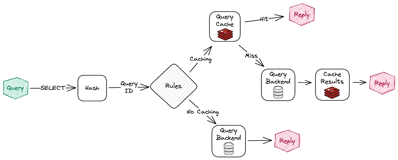
Here is where Redis comes into the picture. It provides tools that expose and accelerate the served data in two ways: caching slow, repeated query results to avoid expensive calls to slower systems (e.g., databases, distributed file systems…) and significantly improving response times using Redis Smart Cache. On the other hand, indexing data in Redis to accelerate querying and providing integration for tools extensively using SQL (e.g., data visualization tools…) by using Redis SQL Trino and Redis SQL ODBC. Let’s see how to use each of these tools.
1 - Redis Smart Cache
As you can imagine from its name, Redis Smart cache uses Redis to cache slow, repeated query results to avoid expensive calls to slower backend systems (e.g., databases, distributed file systems…), improving their response times.
Redis Smart cache works as a wrapper around your backend database’s JDBC driver and puts the SQL queries that are called more often into Cache. Imagine a dashboard that takes a few minutes to refresh because it repeatedly sends the same expansive query to slow backend data stores (HDFS, Oracle…). We all know that distributed systems like HDFS made some tradeoffs regarding latency just to provide high throughput. With Redis Smart Cache, you can still preserve your legacy systems while accelerating their response time considerably.

To use Redis Smart Cache with an existing application, you must add the Redis Smart Cache JDBC driver as an application dependency.
Maven:
<dependency>
    <groupId>com.redis</groupId>
    <artifactId>redis-smart-cache-jdbc</artifactId>
    <version>0.2.1</version>
</dependency>
Gradle:
dependencies {
    implementation 'com. redis:redis-smart-cache-jdbc:0.2.1'
}
Next, set your JDBC URI to the URI of your Redis instance prefixed by JDBC: for example:
jdbc:redis://redis-12000.cluster.redis-serving.demo.redislabs.com:12000
See Lettuce’s URI syntax for all of the possible URI parameters you can use here.
The next step is providing a bootstrap configuration. Redis Smart Cache configuration is done through JDBC properties. The required properties you need to configure are the class name of the backend database JDBC driver you want to wrap up (e.g., oracle.jdbc.OracleDriver) and the JDBC URL for the backend database (e.g., jdbc:oracle:thin:@myhost:1521:orcl). You can also include any property your backend JDBC driver requires, like username or password. These will be passed to the backend JDBC driver as is. For the Smart Cache, you need to configure a few parameters regarding the Redis cache, such as the key prefix for the cached queries, the cache invalidation duration (refresh of the cached queries), cluster configurations like TLS, credentials, the cache capacity… The complete list of Redis smart cache parameters is available here.
Redis Smart Cache uses rules to determine how SQL queries are cached. Rule configuration is stored in a Redis JSON document at the key smartcache:config and can be modified at runtime. In addition, Redis Smart Cache will dynamically update to reflect changes made to the JSON document (see the smartcache.ruleset.refresh property to change the refresh rate).
Here is the default rule configuration:
{
  "rules": [
    {
      "tables": null,
      "tablesAny": null,
      "tablesAll": null,
      "regex": null,
      "queryIds": null,
      "ttl": "1h"
    }
  ]
}
This default configuration contains a single passthrough rule where all SQL query results will be assigned a TTL of 1 hour.
Rules are processed in order, consisting of criteria (conditions) and actions (results). Only the first rule with matching criteria will be considered, and its action will be applied.
- The
tablescriterion triggers if the given tables are precisely the same as the list in the SQL query (order is not important). - The
tablesAnycriterion triggers if any of the given tables appear in the SQL query. - The
tablesAllcriterion triggers if all the given tables appear in the SQL query. queryIdstriggers if the SQL query ID matches any given IDs. An ID is the CRC32 hash of the SQL query. You can use an online CRC32 calculator like this one to compute the ID.regextriggers, if given regular expression, matches the SQL query (e.g., SELECT \* FROM test\.\w*)- Currently, there is only one action available which is
ttl. This parameter sets the time to live for the corresponding cache entries specified in the criteria.
You can also use the Redis Smart Cache CLI that allows managing Redis Smart Cache. While you can configure Smart Cache entirely using JDBC properties, the CLI lets you construct query rules interactively and apply new configurations dynamically. With the CLI, you can also view your application’s parameterized queries or prepared statements and the duration of each query.

After adding the Redis Smart Cache dependency and setting some basic configuration, your JDBC application can take advantage of Redis as a cache without any changes to your code. Let’s try this example to understand how Redis Smart Cache works. This example showcases an application that continuously performs queries against a MySQL database (extensively querying the Products, Customers, Orders, and OrderDetails tables) and uses Redis Smart Cache to cache query results.
If you have a MySQL server installed, you can run this example on your local machine. Or, you can just clone this git repository:
git clone https://github.com/redis-field-engineering/redis-smart-cache.git
cd redis-smart-cache
And use Docker Compose to launch containers for MySQL, Grafana, Redis Stack, and Redis Smart Cache example app instance:
docker compose up
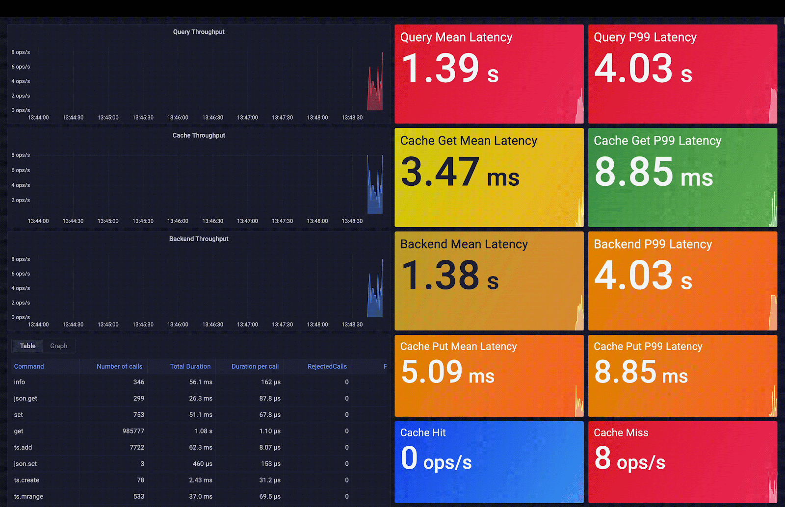
The application starts querying the four tables while joining all of them. Then, for each order with ID x, the query asks the database to sleep x seconds to simulate a slow response time for this query. Conversely, Redis Smart Cache reads the rules from the JSON document at the key smartcache:config and creates a hash data structure containing the SQL query, the queried tables, and the CRC32 hash of the SQL query. Then, caches the query response for each query with the defined TTL.

Once the application uses the Redis JDBC wrapper, It starts querying the backend database transparently. Redis Smart Cache stores the query and its results in the cache if unavailable (missing). When the application calls a query already cached (hit), Redis returns the results stored in the cache with low latency.
Redis Smart Cache captures access frequency, mean query time, query metadata, and additional metrics. These metrics are exposed via pre-built Grafana dashboards; the included visualizations help you decide which query caching rules to apply. As you can observe in the following screenshot, the average query latency passes from 3 seconds (average backend latency) to 0.7 ms (average cache latency), which means an acceleration of 4,200 times the initial latency.
2 - Redis SQL
Like most NoSQL databases in the marketplace, Redis doesn’t allow you to query and inspect the data with the Structured Query Language (SQL). Instead, Redis provides a set of commands to retrieve the native data structures (Key/values, Hashes, Sets…). Still, these commands are not as complete and complex as you can make using SQL (e.g., get the personal data of people having more than 35 years or living in San Fransisco).
For this reason, Redis has developed a module called RediSearch that enables querying, secondary indexing, and full-text search for Redis. These features allow multi-field queries, aggregation, exact phrase matching, numeric filtering, geo-filtering, and vector similarity semantic search on top of text queries.
The idea is to create secondary indices other than the keys (primary ones) and make queries on those indices. For example, we use the FT.CREATE command to create an index on keys prefixed with person: with fields: name, age, and gender. Any existing hashes prefixed with person: are automatically indexed upon creation.
FT.CREATE myIdx
  ON HASH PREFIX 1 "person:"
SCHEMA
  name TEXT NOSTEM
  age NUMERIC SORTABLE
  gender TAG SORTABLE
Now, you can use FT.SEARCH command to search the index for persons with names containing specific words.
FT.SEARCH myIdx "Amine" RETURN 1 name
The previous command returns all persons with names that contain “Amine.” Let’s look for persons older than 35 years in Redis. You can use FT.SEARCH command to search the index for persons with age fields over 35.
FT.SEARCH myIdx "@age:[(35 inf]"
In addition to Redis hashes, you can index and search JSON documents if your database has both RediSearch and RedisJSON enabled.
So far, so good! When your application uses a Redis client library, it will easily search and query the data served by Redis in low latency. Meanwhile, your business analysts are used to the industry standard, SQL. Many powerful tools rely on SQL for analytics, dashboard creation, rich reporting, and other business intelligence work, but unfortunately, they don’t support Redis commands natively. This is where Redis SQL comes in two flavors: Redis SQL JDBC (Trino) and Redis SQL ODBC.
A - Redis SQL JDBC (Trino Connector)
Redis SQL JDBC is a Trino connector that allows access to RediSearch data from Trino. Trino is a distributed SQL engine designed to query large data sets across one or more heterogeneous data sources. It is designed to efficiently query vast amounts of data using distributed queries.
Trino was initially designed to query data from HDFS and has become the obvious choice to query data from anywhere: object storage, relational database management systems (RDBMSs), NoSQL databases, and other systems. Trino was also designed to handle data warehousing and analytics: data analysis, aggregating large amounts of data, and producing reports. These workloads are often classified as Online Analytical Processing (OLAP).
Trino queries data where it lives and does not require a data migration to a single location. Trino can query virtually anything and is truly a SQL-on-Anything system. This means users no longer have to rely on specific query languages or tools to interact with the data in those particular systems. Instead, they can simply leverage Trino, their existing SQL skills, and their well-understood analytics, dashboarding, and reporting tools. These tools, built on top of using SQL, allow the analysis of those additional data sets, which are otherwise locked in separate systems. Users can even use Trino to query across different systems with the SQL they know.

In Trino, the connector-based architecture is at the heart of separating storage and compute: A connector provides Trino an interface to access an arbitrary data source. Each connector provides a table-based abstraction over the underlying data source. As long as data can be expressed in terms of tables, columns, and rows by using the data types available to Trino, a connector can be created, and the query engine can use the data for query processing.
Trino is a SQL query engine that operates similarly to massively parallel processing (MPP) databases and query engines. However, instead of depending on the vertical scaling of a single server, Trino can horizontally distribute all processing tasks across a cluster of servers. This allows for the addition of more nodes to increase processing power.
The Trino coordinator server performs several crucial tasks, including receiving SQL statements from users, parsing them, planning queries, and managing worker nodes. As a central component in the Trino setup, it is the primary point of contact for clients connecting to the Trino installation. Users can interact with the coordinator using the Trino CLI, applications utilizing JDBC or ODBC drivers, or other client libraries available for different programming languages. The coordinator accepts clients’ SQL statements, such as SELECT queries, and processes them for execution.
Trino provides a service provider interface (SPI), an API to implement a connector. By implementing the SPI in a connector, Trino can use standard operations internally to connect to any data source and perform operations on any data source. In addition, the connector takes care of the details relevant to the specific data source.
Redis SQL is a Trino connector that implements the SPI, so Trino can translate the incoming queries (SQL) to the storage concepts of the underlying data source (Redis). For instance, this connector allows making queries to RediSearch indices. Thus, you can query Redis data using SQL and easily integrate with any application compatible with JDBC, such as visualization frameworks like Tableau and SuperSet, and platforms that support JDBC-compatible databases (e.g., Mulesoft).
The coordinator uses the metadata SPI to get information about tables, columns, and types from the underlying data source. For instance, the metadata SPI gets the RediSearch indices (considered as tables), the indexed fields (considered as columns), and the indexed keys returned as rows. These are used to validate that the query is semantically valid and to perform type checking of expressions in the original query and security checks.
The statistics SPI is used to obtain information about row counts (Redis key counts) and table sizes (RediSearch index size) to perform cost-based query optimizations during planning.
The data location SPI is then facilitated in creating the distributed query plan. Finally, it is used to generate logical splits of the table contents.
Once Trino receives a SQL statement, the coordinator is responsible for parsing, analyzing, planning, and scheduling the query execution across the Trino worker nodes. Finally, the statement is translated into a series of connected tasks running on a cluster of workers.
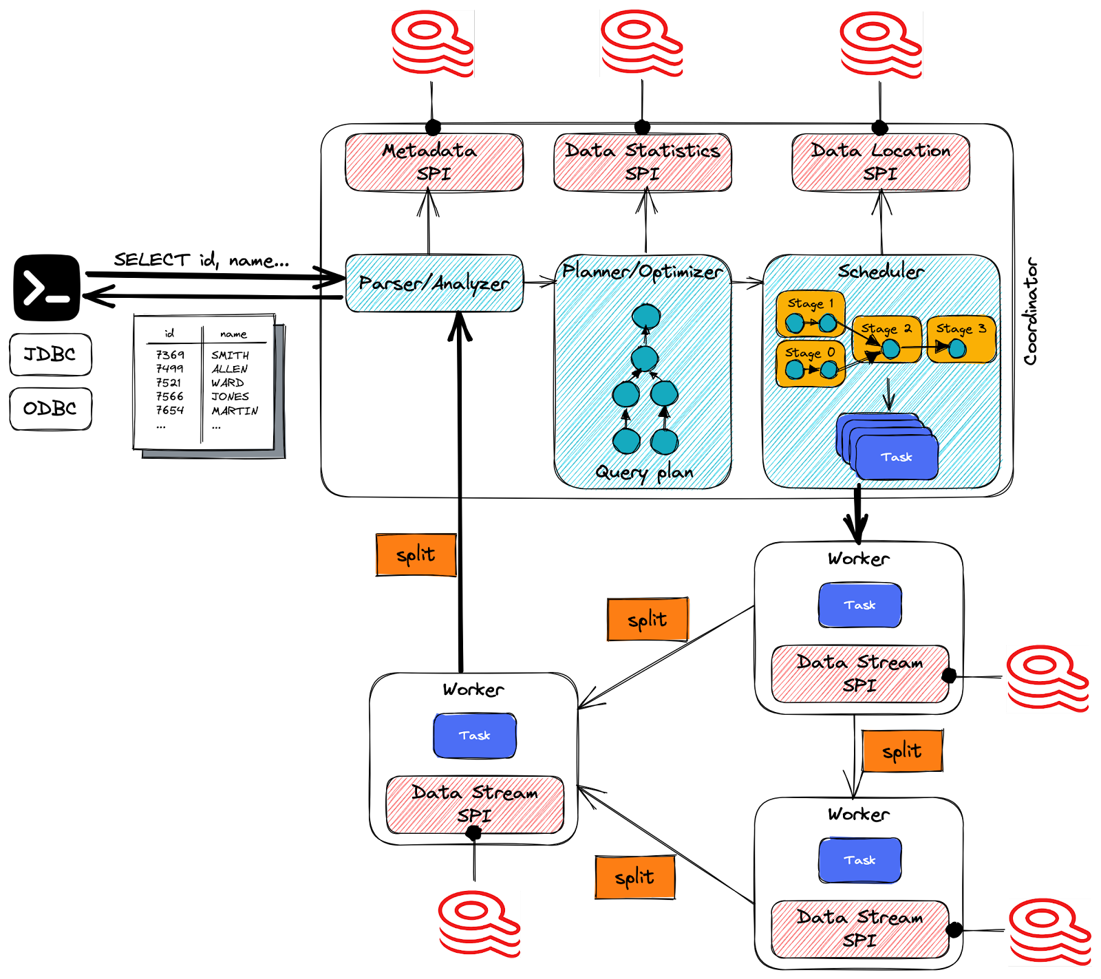
The distributed query plan defines the stages and how the query executes on a Trino cluster. It’s used by the coordinator to further plan and schedule tasks across the workers. A stage consists of one or more tasks. Typically, many tasks are involved, and each task processes a piece of the data.
Splits are the smallest unit of work assignment and parallelism that a task processes. A split is a descriptor for a segment of the RediSearch data that a worker can retrieve and process. It is here where the magic happens! The specific operations on the data performed by the connector are simply the RediSearch-specific queries (e.g., FT.SEARCH).
As the workers process the data, the results are retrieved by the coordinator and exposed to the clients on an output buffer. Once an output buffer is completely read by the client, the coordinator requests more data from the workers on behalf of the client. The workers, in turn, interact with the data sources to get the data from them. As a result, data is continuously requested by the client and supplied by the workers from the data source until the query execution is completed.
Let’s see how it works in practice. First, consider this file, which contains an organization’s general ledger. A general ledger represents the record-keeping system for a company’s financial data, with debit and credit account records. It provides a record of each financial transaction that takes place during the life of an operating company and holds account information needed to prepare the company’s financial statements. Each financial transaction is associated with an accounting number (ACCOUNTNUM).
In most organizations, the accounting numbers are part of a Chart of Accounts (CoA). A chart of accounts lists the names of the accounts that a company has identified and made available for recording transactions in its general ledger. A company can tailor its chart of accounts to best suit its needs, including adding accounts as needed. Consider the Chart of Accounts that lists the accounts used in the general ledger presented previously and the Accounting Nature table, which groups the accounts by nature (Asset, Equity, or Liability)

First, let’s ingest these three tables using the RIOT-file tool. For install procedure and configuration, see Data & Redis - Part 1
We will ingest and integrate the General Ledger table as Hashes in Redis. For this, run the following command:
riot-file -h redis-12000.cluster.redis-serving.demo.redislabs.com -p 12000 -a redis-password import https://raw.githubusercontent.com/aelkouhen/aelkouhen.github.io/main/assets/data/GeneralLedger.csv --header hset --keyspace GeneralLedger --keys RECID
We do the same for the other tables, Chart of Accounts and Accounting Nature.
riot-file -h redis-12000.cluster.redis-serving.demo.redislabs.com -p 12000 -a redis-password import https://raw.githubusercontent.com/aelkouhen/aelkouhen.github.io/main/assets/data/ChartAccounts.csv --header hset --keyspace CoA --keys ACCOUNTNUM
riot-file -h redis-12000.cluster.redis-serving.demo.redislabs.com -p 12000 -a redis-password import https://raw.githubusercontent.com/aelkouhen/aelkouhen.github.io/main/assets/data/AccountingNature.csv --header hset --keyspace AccountingNature --keys AccountingNatureCode
Once you have your data ingested into Redis. You can create secondary indices on the three tables:
general_ledger as a secondary index for the General Ledger table. We need Only the Account Number, the Transaction Amount (AMOUNTMST), and the Currency Code to be indexed.
FT.CREATE general_ledger
  ON HASH
    PREFIX 1 "GeneralLedger:"
  SCHEMA
    ACCOUNTNUM TEXT SORTABLE
    AMOUNTMST NUMERIC SORTABLE
    CURRENCYCODE TAG SORTABLE
chart_accounts as a secondary index for the Chart of Accounts table.
FT.CREATE chart_accounts
  ON HASH
    PREFIX 1 "CoA:"
  SCHEMA
    ACCOUNTNUM TEXT SORTABLE
    Description TEXT NOSTEM
    Nature TEXT SORTABLE
    Statement TAG SORTABLE
    AccountingNatureCode TAG SORTABLE
And accounting_nature as a secondary index for the Accounting Nature table.
FT.CREATE accounting_nature
  ON HASH
    PREFIX 1 "AccountingNature:"
  SCHEMA
    AccountingNatureCode TAG SORTABLE
    AccountingNature TEXT SORTABLE
    Description TEXT NOSTEM
    AccountGroup TAG SORTABLE
Now, you can test these indices by running the following commands:
FT.SEARCH general_ledger "@AMOUNTMST:[(100000 inf] @CURRENCYCODE:{EUR|USD}"
FT.SEARCH chart_accounts "@ACCOUNTNUM:61110801"
FT.SEARCH accounting_nature "@AccountGroup:{Payables|Receivables}"
The first query returns the financial transactions over 10,000 euros or u.s. dollars. The second one returns details on account number 61110801. Finally, the last query returns all the Payables1 and Receivables2 account numbers. You can observe that using RediSearch commands is not evident for data engineers and may turn out to be a huge headache if you want to perform complex queries.
Now, let’s run the Trino CLI to figure out quickly that executing SQL queries is much easier and simpler:
trino --catalog redisearch --schema default
Let’s try the same previous RediSearch queries with SQL syntax using Redis SQL Trino.

Let’s try a more advanced query similar to those executed in the analytics workloads. We use Redis SQL Trino to make joins and some windowing functions between the three RediSearch indices: I would ask to get the sum of all Receivable and Payable transactions in the general ledger. For this, you need to join general_ledger to chart_accounts through the AccountNumber, join chart_accounts to accounting_nature to be able to group and sum the transactions amounts by the AccountingGroup, then filter the results to select only transactions related to Receivables and Payables.

The most practical use case using Redis SQL Trino is connecting data visualization tools to a low latency data store like Redis. In fact, Redis is an in-memory data store, and Its power resides in its ability to serve data with the fastest possible response times.
For this reason, Redis is frequently used as a serving layer in data pipeline architectures (e.g., kappa architectures, online feature stores, etc.) and for caching OLAP application queries to accelerate response time.
For instance, to improve data visualization performance (e.g., while refreshing analytics dashboards and reports), you can use Redis to store the datasets that are most frequently queried, create secondary indices on them using RediSearch, then benefit from the Trino connector for RediSearch to leverage SQL queries instead of RediSearch commands.
The following is an example of a JDBC URL used to create a connection from Tableau to Redis SQL Trino
jdbc:trino://localhost:8080/redisearch/default

B - Redis SQL ODBC
ODBC (Open Database Connectivity) is an interface specification that allows applications to access data from various database management systems (DBMS) using a common set of function calls. ODBC is part of the Microsoft Windows Open Services Architecture (WOSA), which provides a way for Windows-based desktop applications to connect to multiple computing environments without requiring any modification to the application.
ODBC is based on the Call Level Interface (CLI) specification from SQL Access Group and provides a set of API functions that allow developers to interact with a wide range of DBMSs, including Microsoft SQL Server, Oracle, MySQL, and of course, Redis.
Redis SQL ODBC is a native ODBC driver that lets you seamlessly integrate Redis with Windows-based desktop applications like Microsoft Excel or Power BI. Just like the other tools presented before, this tool may dramatically improve your Power BI query response times. With the Redis SQL ODBC driver installed, Power BI can perform single-table queries against secondary indexes (RediSearch) across Redis hashes or JSON documents in real-time.

Redis SQL ODBC takes the SQL generated by the end-user applications, such as Power BI, translates it into the RediSearch query language, performs the query across Redis hashes or JSON documents using secondary indexes, and then arranges the results back into an ODBC-compliant result set for consumption by the frontend.
Integrating Redis SQL ODBC with Windows-based desktop applications requires only a small configuration change. All you need is to install the driver by downloading the installer pack from the latest release of Redis SQL ODBC. Unzip it, and then run the included .msi file. Then follow the steps from the MSI to install the driver.
Then you can set up the Redis data source, by running:
1. the following command in PowerShell (Windows 10+) and substituting host, port, username, and password with the appropriate credentials.
Add-OdbcDSN -Name "Redis" -DriverName "Redis" -Platform "64-bit" -DsnType "User" -SetPropertyValue @("host=hostname", "port=portNum", "username=username", "password=password")
Here, I reuse the same database as the last section (Trino):
Add-OdbcDSN -Name "Redis" -DriverName "Redis" -Platform "64-bit" -DsnType "User" -SetPropertyValue @("host=redis-12000.cluster.redis-serving.demo.redislabs.com", "port=12000", "username=default", "password=redis-password")
2. Or, with the ODBC data sources GUI:

For this tool, we’re going to load a funny dataset! Tim Renner put together a dataset on data world with a bunch of UFO sightings – we’ll load that dataset into Redis, using RIOT-File (see Data & Redis - Part 1) and see what we can do with it using some Windows-based desktop applications.
$ riot-file -h redis-12000.cluster.redis-serving.demo.redislabs.com -p 12000 -a redis-password import https://raw.githubusercontent.com/aelkouhen/aelkouhen.github.io/main/assets/data/nuforc_reports.csv.gz --process id="#index" --header hset --keyspace Report --keys id
Then, we will create a secondary index on ingested reports created by the last command::
FT.CREATE ufo_report
  ON HASH
    PREFIX 1 "Report:"
SCHEMA
  shape TEXT SORTABLE
  city TEXT SORTABLE
  state TEXT SORTABLE
  country TEXT SORTABLE
  city_longitude NUMERIC SORTABLE
  city_latitude NUMERIC SORTABLE
Let’s test the Redis ODBC driver with a Microsoft Excel Sheet. First, we run “get data from another source” in the Data menu, then choose the menu “from an ODBC driver”.
Next, we choose the Redis data source in the prompt and put the SQL query we want to execute against the secondary index. Now we can query data across our Redis Enterprise database. In our case, we have a RediSearch index called ufo_reports, representing the stored UFO sightings reports.

Now that we’ve analyzed our data in Microsoft Excel, we can create some basic visualizations/charts in Excel itself, or we can leverage our ODBC driver to make more advanced data visualizations in Power BI. Similarly to Excel, you can load data in Power BI by choosing the menu “Get Data From another Data Source” or by clicking to the “Get Data” drop-down menu and press “More…” In addition, you can choose to transform data and perform some filtering on loaded data.
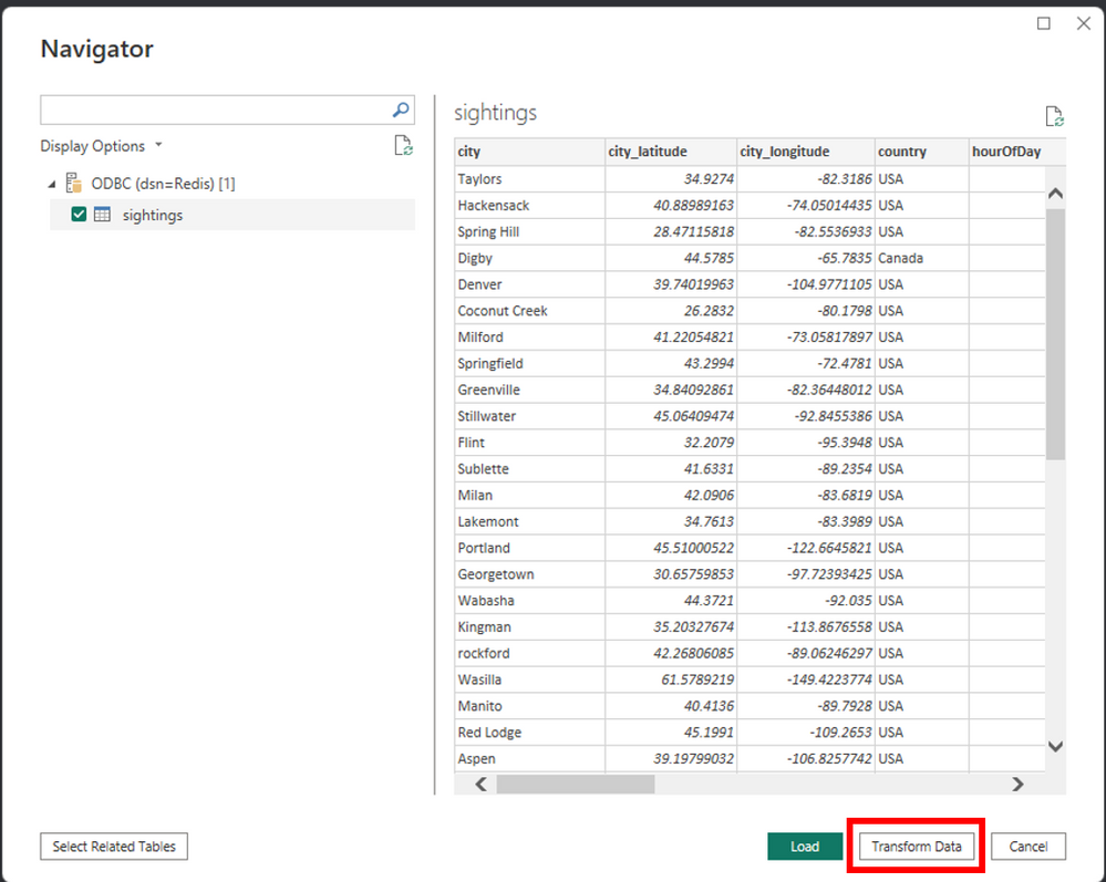
You can filter your data from the Power Query Editor and select which columns you want to load. For example, let’s filter the states down to Florida: First, click the arrow next to the state column and then “(Select All)” to de-select all the states. Next, click the checkbox next to “FL” to filter down to Florida. Then click “OK” to finish the filtering. Now that we loaded all our “sightings” data into Power BI, let’s build a dashboard to visualize our data.

This walkthrough shows that Redis SQL ODBC is a seamless integration between Redis and Power BI. With it, we can bring the speed and efficiency of Redis to our reporting using the venerable ODBC standard.
Machine Learning
The second significant area of data serving is machine learning (ML). With the emergence of ML engineering as a parallel field to data engineering, you may wonder where data engineers fit into the picture. But to be aligned with the state of the art, data engineers’ main role is to provide data scientists and ML engineers with the data they need to do their job. In the following posts, I’ll introduce in more detail the tools and capabilities provided by Redis to serve machine learning applications. Briefly, the most common ways to serve Redis data for Machine Learning applications are:
1. File exchange is quite a common way to serve data. Curated data is processed and generated as files to consume directly by the final users. For example, a business unit might receive invoice data from a partner company as a collection of CSVs (structured data). A data scientist might load a text file (unstructured data) of customer messages to analyze the sentiments of customer complaints. We have used RIOT in Data & Redis - Part 1 as a batch ingestion tool. We often used the import parameter to load data into Redis. However, RIOT-File also allows exporting (export command) data from Redis as a delimited, JSON, or XML File. You can also export data in batches from Redis as AWS S3 objects or GCP Storage objects.
2. Databases can play the role of AI feature stores. A feature store is a centralized repository specifically designed for managing, storing, and sharing the features used in machine learning models. In machine learning, features are the input variables or predictors that train models to make predictions or classifications. The feature store enables data scientists and engineers to store, discover, share, and reuse features across different models and applications, improving collaboration and productivity. In future posts, I’ll use Redis as a Feature Store for a few Machine Learning applications, such as Recommendation Engines or Fraud Detection Applications.
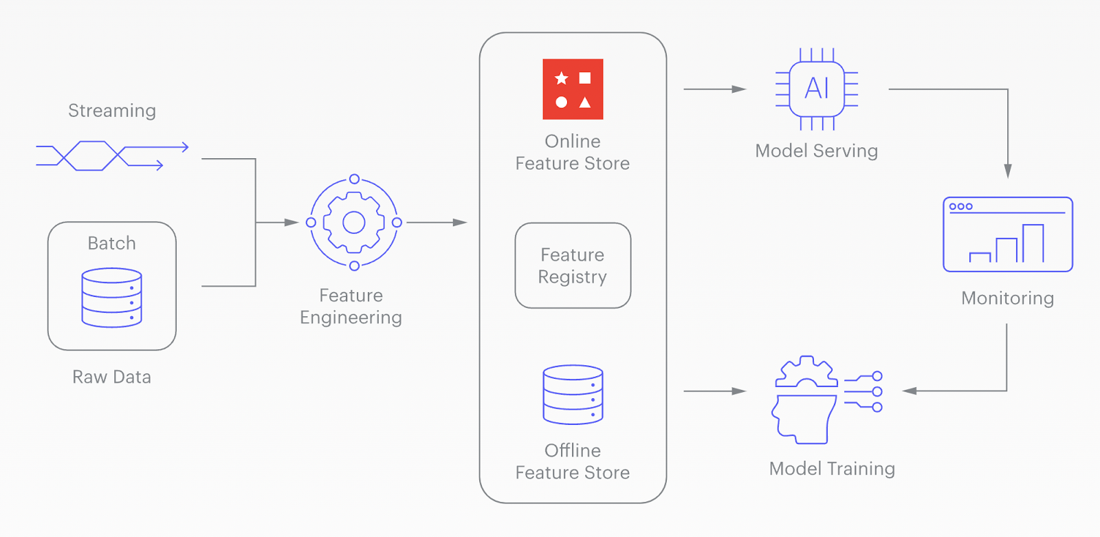
Another way to serve data for ML is through vector databases. A vector database is a type of feature store that holds data in vectors (mathematical representations of data points). Machine Learning algorithms enable this transformation of unstructured data into numeric representations (vectors) that capture meaning and context, benefiting from advances in natural language processing and computer vision.

Vector Similarity Search (VSS) is a key feature of a vector database. It finds data points similar to a given query vector in a vector database. Popular VSS use-cases include recommendation systems, image and video search, natural language processing (like ChatGPT), and anomaly detection. For example, if you build a recommendation system, you can use VSS to find (and suggest) products similar to a product in which a user previously showed interest. In the following posts, I’ll introduce Redis as a vector database for machine learning applications, such as Sentiment Analysis or Conversational ChatBots.
3. Data virtualization engines: In the previous sections, We have seen various Redis tools that allow data virtualization. For example, the Redis SQL suite (both JDBC and ODBC) provides a way to perform federated queries: where data is pulled from Redis secondary indexes, then exposed to systems and applications that use SQL queries.
Reverse ETL
Nowadays, Reverse ETL is a popular term that refers to loading data from a downstream database back into a source system. For example, a data engineer may extract customer and order data from a CRM and store it in a data warehouse to use it for training a lead scoring model. The model’s results are then stored back in the data warehouse. The company’s sales team intends to use these scored leads to boost sales and hence requires access to them. Using reverse ETL and loading the scored leads back into the CRM is the easiest approach for this data product. Reverse ETL takes processed data from the output side of the data journey and feeds it back into source systems.
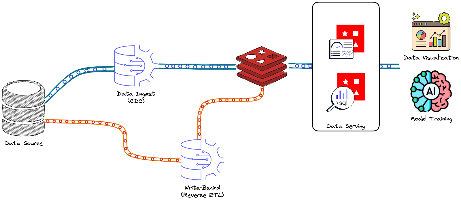
In Data & Redis - Part 4, we have seen the Write-Behind policy provided by Redis Data Integration (RDI). In this scenario, data is synchronized in a Redis DB and pushed back to some data sources. In fact, this policy can be considered a Reverse ETL process since you can think about it as a pipeline that starts with curated data in Redis and then filters, transforms, and maps it to the source data store data structures. However, RDI Write Behind is still under development and supports only the following data stores: Cassandra, MariaDB, MySQL, Oracle, PostgreSQL, and SQL Server.
Summary
The serving stage is about data in action. But what is a productive use of data? To answer this question, you need to consider two things: what’s the use case, and who’s the user?
The use case for data goes well beyond viewing reports and dashboards. High-quality, high-impact data will inherently attract many exciting use cases. But in seeking use cases, always ask, “What action will this data trigger, and who will be performing this action?” with the appropriate follow-up question, “Can this action be automated?” Whenever possible, prioritize use cases with the highest possible ROI.
Now that we’ve taken a journey through the data journey, you know how to design, architect, build, maintain, and improve your data products using Redis Enterprise. In the following posts, I’ll turn your attention to the most used use-case of Redis as a real-time data platform. This will involve an end-to-end data journey applying everything you have learned in this series.
References
- A. I. Maarala, M. Rautiainen, M. Salmi, S. Pirttikangas and J. Riekki, “Low latency analytics for streaming traffic data with Apache Spark,” 2015 IEEE International Conference on Big Data (Big Data), Santa Clara, CA, USA, 2015, pp. 2855-2858, doi: 10.1109/BigData.2015.7364101.
- M. Fuller, M. Moser, M. Traverso, “Trino: The Definitive Guide”, 2nd Edition, O’Reilly Media, Inc. ISBN: 9781098137236
- Redis Smart Cache, Redis.
- Redis SQL Trino, Developer Guide.
- “How to use Redis as a Data Source for Power BI with Redis SQL ODBC”, Microsoft Azure Blog.
- Features Store, Redis Blog.
- Vector Database, Redis Blog.
- Redis Data Integration (RDI), Developer Guide.
1. Account Payables (AP): a company’s short-term obligations owed to its creditors (e.g., suppliers) still need to be paid.
2. Account Receivables (AR): the money a company’s customers owe for goods or services they have received but not yet paid for.